Manajemen | Fakultas Ekonomi Universitas Maritim Raja Ali Haji 073500104000000172

(1)

Full Terms & Conditions of access and use can be found at

http://www.tandfonline.com/action/journalInformation?journalCode=ubes20

Download by: [Universitas Maritim Raja Ali Haji] Date: 13 January 2016, At: 00:30

Journal of Business & Economic Statistics

ISSN: 0735-0015 (Print) 1537-2707 (Online) Journal homepage: http://www.tandfonline.com/loi/ubes20

Semiparametric Approaches to Welfare

Evaluations in Binary Response Models

Walter Belluzzo Jr

To cite this article: Walter Belluzzo Jr (2004) Semiparametric Approaches to Welfare Evaluations in Binary Response Models, Journal of Business & Economic Statistics, 22:3, 322-330, DOI: 10.1198/073500104000000172

To link to this article: http://dx.doi.org/10.1198/073500104000000172

View supplementary material

Published online: 01 Jan 2012.

Submit your article to this journal

Article views: 49

(2)

Semiparametric Approaches to Welfare

Evaluations in Binary Response Models

Walter B

ELLUZZO

, Jr.

Department of Economics, University of São Paulo at Ribeirão Preto, 14.040-900 Ribeirão Preto, São Paulo, Brazil (belluzzo@usp.br)

Applied welfare analysis is commonly based on mean or median benet estimates. However, the whole conditional distribution of benets is often of interest for policy makers. This article compares the distrib-utional information recovered by competing semiparametric methods. Results obtained using a valuation study for the improvement of water resources in Brazil suggest that the semiparametric approaches are in line with each other, capturing a rich heterogeneity structure that is ignored by the logit approach. Failure to take this structure into account may lead to the undue rejection of the project according to the Kaldor–Hicks criterion.

KEY WORDS: Binary quantile regression; Contingent valuation; Klein and Spady estimator; Semipara-metric methods; Water resources.

1. INTRODUCTION

To date, applied welfare analysis of public expenditure projects through binary response valuation models seems restricted to estimates of the mean or median benets. Even though the focus on mean or median estimates is justied by the Kaldor–Hicks and the voting criteria (Hanemann 1989), policy makers may be interested in a myriad of other aspects of a project. In particular, they are often interested in identi-fying those who are affected, as well as how much each in-dividual is affected. For this reason, in addition to the mean and median, the whole conditional willingness-to-pay distribu-tion constitutes valuable informadistribu-tion to policy makers. It facil-itates adjusting project implementation according to whatever weighting scheme is implied by their policy objectives.

In binary response valuation models, this distributionalinfor-mation cannot be retrieved directly, due to the latent nature of willingness to pay. This aspect of willingness to pay favors es-timating a conditional mean function with parametric assump-tions about the underlying distribution. The problem with such a modeling approach is that welfare evaluations, which depend crucially on the shape of the underlying distribution, are deter-mined to a great extent by ad hoc assumptions. In this context, distribution-freesemiparametric methods provide an interesting alternative modeling approach, because they make it possible to impose some structure as well as to recover important distribu-tional information from data.

Several distribution-free models are available for estimating binary response models (Manski 1975; Cosslett 1983; Klein and Spady 1993; Horowitz 1992). Applications of these meth-ods to valuation models are not numerous, however. Appar-ently, only Creel and Loomis (1997), Chen and Randall (1997), and Li (1996) have considered distribution-free methods for the estimation of valuation models. Nonetheless, evidence from this literature seems to indicate that semiparametric and the usual parametric methods provide similar parameter estimates at the center of the willingness-to-pay distribution (Li 1996).

This similarity of estimates at the center of the distribution suggests that if the main interest is to evaluate a project ac-cording to the Kaldor–Hicks or the voting criteria, the choice of an estimation method may be of minor importance. Clearly, however, the same is not true if the main interest is in assessing

distributionalinformation about the welfare impact of a project. Even if the mean and median willingness-to-pay estimates are similar, the implied shape of the distribution may vary con-siderably between methods, with important consequences for project evaluation.

The purpose of this article is to provide a comparison of the willingness-to-pay distribution implied by competing semi-parametric methods for the estimation of binary response mod-els. Specically, two methods are compared: Klein and Spady’s (1993) estimator (KSE) and Kordas’s (2000) smoothed binary regression quantiles (SBRQ) estimator. The comparison is de-veloped in terms of estimates of the proportion of losers and the expected gains at various covariate levels. Because these wel-fare measures are directly related to the implied willingness-to-pay distribution, the comparison of welfare measures obtained through different methods may be viewed as equivalent to a comparison of the implied conditional distributions.

The data used for the comparison of welfare measures in-volve an application of the contingent valuation to a project for management and improvement of an important Brazilian river basin, the Paraíba do Sul, by the residents of the metropolitan area of Rio de Janeiro. The project is closely related to fed-eral legislation for the management of water resources in Brazil, which requires the creation of an administrative agency respon-sible for investment plans and the corresponding nancing as-pects. The benets of project implementation include reduced pollution levels of the basin’s rivers, improved outdoor activi-ties in the areas surrounding the basin’s rivers including some parks, and especially maintained/improved domestic tap water supply and sewage collection.

2. BINARY RESPONSE VALUATION MODEL

This section introduces the binary response model associ-ated with the contingent valuation method. To keep the gen-eral context clear, consider a simplied example. Suppose that the project to be valued implies a xed cost equally shared by

322

(3)

Belluzzo: Welfare Analysis 323

all individuals, so that it generates both gainers and losers at a given cost share. Suppose that a contingent valuation study for this project is implemented with the elicitation question in thereferendumformat: “Would you be willing to pay $tfor the implementation of this project?” Each individual faces a bid value,t, randomly drawn from a pool ofTbids.

This preference revelation mechanism is connected to eco-nomic theory by the association of the bid value with a Hicksian measure of welfare change. The correct measure depends on the specic way in which the referendum question is formu-lated (Mitchell and Carson 1989). To simplify the exposition, I focus on the compensating variation, which in this case cor-responds to the dollar amount that should be taken from an individual to keep him or her at the initial utility levelafter

project implementation. As a result, a “yes” answer can be in-terpreted as meaning that the bid value,t, is less than or equal to the compensating variation associated with the project. Because the compensating variation can be written in terms of a differ-ence of expenditure functions, it follows that a “yes” answer implies that

s.m;AIµ/De¡0;v.0;m;AIµ/¢¡e¡1;v.0;m;AIµ/¢¸t;

whereµ is a vector of parameters,mis income,Ais a vector of individual’s characteristics. The functionv.j;¢/is the indirect utility function, withjD1 if the project is implemented and

jD0 if it is not. Finally,e.j;¢/Dv¡1.j;¢/is the expenditure function. For future reference, the functions.m;AIµ/will be called thevaluation function.

The characterization of the unobserved true willingness to pay,y¤, as a random variable can be obtained by introducing a random term,", in the valuation function,

y¤_i Ds.xi;µ/C"i; "i»F"i; (1)

wherex´ fm;AgandF"is the distribution function of". Then a binary response valuation model can be written as

yiD

»

1 ify¤_i ¸ti

0 otherwise. (2)

In general, the estimation of the binary response valuation model given in (2) depends on assumptions regardingF" and the functional form ofs.xi;µ/. The distributional assumptions

underlying the estimation methods are crucial for computing welfare measures. As discussed later, these welfare measures are dened as functionals of the conditional willingness-to-pay distribution. Consequently,differences in the underlyingF" may lead to biased welfare measures.

Regardless of the estimation method, several welfare mea-sures can be dened from the underlyingF". The main interest in this article is the proportion of losers and the expected gains and losses, conditional on income ranges. These measures can be dened as follows. To avoid any confusion with the bid val-ues,t, letcbe the individual cost share of the project. Then, for any givenxand any cost sharec, the proportion of gainers can be obtained directly by computing

P1j_x;cD with¯1D®. Then the conditional expectation of positive gains (gains) can be written as

GC.x;c/D Z 1

¡1

G.x;c/ ¡G.x;c/¸0¢dF"j_x: (4)

SubstitutingG._x;c/ <0 for the inequality in the indicator func-tion (4) gives the condifunc-tional expectafunc-tion of negative gains (losses), denoted byG¡.x;c/. Provided that there is sufcient information aboutF", (3) and (4) can be used to obtain esti-mated welfare measures conditionalon any vector of individual characteristics,x, and cost,c. In practice, however, specifying and reporting all individual characteristics generally is not fea-sible. A better approach in the present case may be to group individuals according to a few income ranges. In some sense, this is equivalent to focusing on a typical individual for each income range.

Focusing on typical individual for each income range also facilitates aggregating gains and obtaining unconditional ex-pected gains; aggregate exex-pected gains for each range can be obtained by multiplying the individual gains by the number of individuals in each range. Unconditional gains can be approxi-mated by summing gains over ranges, which can be viewed as simplistic way of integrating outxin (4).

3. ESTIMATION METHODS

3.1 Censored Logit

Introduced by Cameron (1988) as an analog of a censored regression, the censored logit is based on the specication of a conditional mean model for the unobserved willingness to pay. Specically, assuming thatE."j_x/D0, it follows directly from (1) thatE.y¤jx/Ds.x;µ/.

Parametric estimation of conditionalmean models associated with (2) can be implemented as the optimization of the log-likelihood function where¾ is a scale parameter (Cameron 1988).

Note that in this parametric setting, any welfare measure can be easily computed. Because F" is given by assumption, the conditional mean and scale estimates can be used to compute any functional of the conditionaldistribution ofy¤. Specically, the integrals in (3) and (4) can be computed directly for logis-tic F"jx, yielding welfare measures conditional on any set of

individual characteristics.

But it is important to stress that even though one can obtain any welfare measures of interest from the censored logit model, ifF"is misspecied and/or the iid error assumption is violated, then the results obtained are likely to be poor. In fact, as the results presented in Section 4 suggest, logit estimates may lead to the undue rejection of the project.

(4)

3.2 Klein and Spady Estimator

The main idea of Klein and Spady’s (1993) estimator is to replace the probabilitiesF.z/in the likelihood function (5) by a nonparametric estimate,FO.z/. To obtain this nonparametric estimate, these authors noted that the true probabilitiesF.z/can be written in terms of the density ofzconditional ony, denoted byg.zjy/. Specically, for any realz, the true probability can be written as

F.z/D Pg.zjyD1/

Pg.zjyD1/C.1¡P/g.zjyD0/; (7)

where PDPr[yD1]. Because g.y;z/´Pg.zjy/, Klein and Spady proposed obtainingFO.z/using kernel estimates of the joint densitiesgyzDg.y;z/. For the standard normal density as

the kernel function,gyzcan be estimated by

O

where Á is the standard normal density,hN is a sequence of

bandwidths satisfying Nh6_N ! 1and Nh8_N !0 as N! 1, and¸Oyj is a local smoothing parameter. Specically, for a

pi-lot bandwidth,hNP, letOlyj´ Ogyz.zjI1;µIhNP/be a preliminary

density estimate. Then the local smoothing parameter is de-ned as ¸OyjD O¾y.µ/.Olyj=m/¡1=2, where ¾Oy.µ/ is the standard

deviation of zconditional on yand mis the geometric mean ofOlyj. [See Klein and Spady (1993) for the denition of

bias-removing bandwidth.]

The estimator ofµcan be obtained by maximizing the quasi-likelihood function whereFO is obtained by substituting the estimates (8) into (7). Klein and Spady (1993) provided the asymptotic theory of the KSE based on a trimmed version of the estimator. Speci-cally, they showed that this estimator is consistent and attains Cosslett’s (1987) efciency bound. In addition,N1=2times the centered estimator of¯ is asymptotically normal. In general, trimming has little effect on the estimates and thus may not be necessary in some applications (Horowitz 1993a). Because in the application of Section 4, estimates are not affected by trim-ming, only the untrimmed estimator was presented.

For a linear index,®Cx0i¯¡ti, the intercept is not identied

in Klein and Spady’s model. Rather, it is assimilated into the random error term. Even though it can be estimated using an adaptation of the procedure that Li (1996) proposed for the in-tercept estimation in Cosslett’s (1983) model, it sufces for the development of welfare measures to note that the probability ofyD0 can be written as

Pr.x0i° ¡·ti·´/´F´.x0i° ¡·ti/DF"¤.®¡x 0

i¯¡ti/; (10)

where ·´1=¾,´D· ."C®/, and° D·¯. The notationF_"¤

indicates that this distribution is scaled by a function s, that captures unspecied heterogeneity.

It follows from (10) that estimates of the proportion of losers and expected gains can be computed directly usingFO´. In par-ticular, the proportion of gainers can be estimated directly from

(7) and (8), whereas estimates of the expected gains can be ob-tained approximating the integral (4) by

O

whereti is an increasing sequence of costs, preferably not far

from the observed bid values. Likewise,xandc dening the evaluation pointziof (8) should not be far away from the sample

observed values. Out-of-sample predictions without parametric assumptions are always unreliable (Cosslett 1983, p. 771). The expected losses can be estimated by substitutingc<ti for the

inequality in the indicator function (11).

3.3 Smoothed Binary Regression Quantiles

Instead of specifying a willingness-to-pay conditional mean function, I now consider the specication of the willingness-to-pay conditional quantile functions. For a given¿ 2.0;1/, let Qy¤.¿jx/ be the ¿th quantile of the true willingness to pay,y¤, conditional onx. Then, assuming that the conditional quantiles ofy¤assume a linear form given byx0¯.¿ /, I can write

If y¤ could be observed directly, then the preference pa-rameters would be readily estimable through Koenker and Bassett’s (1978) quantile regression method. Buty¤is not ob-servable; only the transformation .y¤_i ¸ ti/ is observed. In

such a case, an estimable model can still be specied using the quantile’s equivariance to monotone transformations: for any monotoneh:R!R, it follows thath.Qy.¿jx//DQh.y/.¿jx/,

As was shown by Kordas (2000), the model (14) can be estimated through an extension of Horowitz’s (1992) median smoothed maximum score. Using the standard normal distri-bution function as the kernel, the smoothed binary regression quantiles can be written as

max

where8represents the standard normal cdf andhN is a

band-width sequence satisfying limN!1hND0.

Horowitz (1992) provided a comprehensive asymptotic the-ory for the estimator with ¿ D:5, including methods for consistent estimation of standard errors, removal of asymptotic bias, and bandwidth selection. The extension of Horowitz’s re-sults to general quantiles was introduced by Kordas (2000). Specically, the centered bias-corrected estimator is normally distributed and strongly consistent under general assumptions. The rate of convergence is shown to be at least as fast asN¡2=5 and can be arbitrarily close toN¡1=2, depending on the smooth-ness of the distributions of"andx0¯.¿ /.

For the binary regression quantiles, computation of welfare measures requires rewriting (3) and (4) in a convenient form.

(5)

Specically, as suggested by Kordas (2000), variables can be changed so that¿ DF"j_xand (3) can be rewritten as

Kordas’s (2000) approximation,M¡1PM

mD1 .x0¯.¿m/¡c/,

which implicitly assumes equally spaced quantiles over the en-tire.0;1/range.

For computation of gains and losses, in addition to the change in variables, it is necessary to dene quantile-specic gains,

G.¿jx;c/´x0¯.¿ /¡c. Then the conditional expectation of positive gains givenxandccan be written as

GC.x;c/D dicator function (18) gives the expression for the conditional expectation of negative gains (losses), denoted by G¡.x;c/. These expectations can be approximated using a grid of quan-tiles, as indicated in (17). Specically, the lower bound of the expected positive gains, (18), may be estimated by

O

pected losses may be estimated by

O

The approximations in (19) and (20) provide a convenient way to clarify the derivation and interpretation of the corre-sponding integrals. Suppose thatGOC_mD:75 andGOC_m_¡₁D:60 for a given.x;c/pair. Then, by construction, it is clear that 75% of the individuals characterized by x would have gains less thanGOC_m when the cost share is c. Similarly, 60% of the in-dividuals would have gains less thanGOC_m_¡₁. As a result, there is a total of 1¿m D15% of individuals whose gains would

be at most GOC_m and at least GOC_m_¡₁. At this point it should be clear that (19) is nothing but a weighted average of the gains for a givenx and c. Also, noting that¿ DF"j_x, it

be-comes clear that (19) approximates the area aboveF"jx and

to right ofc, which corresponds to the expected value dened in (18). The same reasoning applies to the denition of the ex-pected losses.

To conclude this section, I discuss the relative merits of the three models presented earlier. The balance of the restric-tive distributional assumptions underlying the logit model is its computational simplicity. The two semiparametric models considered in this article are not nested within each other. Nonetheless, as pointed out by an anonymous referee, some

heuristic comparisons can still be made. The Klein and Spady (1993) model can accommodate unspecied heterogeneity that depends on x only through the single index. The quantile re-gression model, in contrast, allows more general forms of het-erogeneity in that each conditionalquantile function is specied separately. The balance of the quantile models discussed earlier is the linearity of quantile functions, because it implies that they will cross in the presence of heterogeneity. In general, the crossing of quantile functions is not an issue if it occurs out of the sample range, but any crossings within the sample range should be handled by the monotone-constrained smoothing dis-cussed later.

Finally, both semiparametric approaches are more demand-ing in terms of bid design. In particular, the identication of the tails of the willingness-to-pay is possible only to the extent that there are bid values that carry relevant information about these portions of the distribution.Obviously, the presence of bid values far into the tails of the willingness-to-pay distribution is not an issue in the logit model.

4. DATA AND ESTIMATION RESULTS

4.1 Data

The application of the contingent valuation method analyzed in this article involves the valuation of a project for manage-ment and improvemanage-ment of an important Brazilian river basin, the Paraíba do Sul. The complete study contains two inde-pendent samples, the rst sample corresponding to the region within the boundaries of the river basin and the second corre-sponding to the Rio de Janeiro metropolitan area, which, even though located out of the boundaries of the river basin, receives most of its tap water supply from the river basin. To facilitate retrieving the populational data required by the proposed meth-ods, I analyze only the Rio de Janeiro sample in this article.

The Paraíba do Sul river is located in southeast Brazil, in a region of high population and industrial concentration. Conse-quently, the basin’s rivers face increasing demands, and their general condition has suffered a steady deterioration over time. The project being valued involves investments intended to pre-serve the areas that still are in good condition and to recover those areas already compromised, according to proposed fed-eral legislation for the management of water resources in Brazil. The institutional arrangement of the project includes the cre-ation of an administrative agency, with the role of determining and implementing investment plans and the cost share for all consumers, domestic and industrial. This close relation with proposed legislation is important, for it considerably reduces the hypothetical nature of the scenario being presented to the interviewees.

In general, the descriptions of the investments are very tech-nical, and their relationships to concrete benets are not direct in most cases. For this reason, the scenarios were designed to focus on benets rather than description of investments, which were substituted by a more general characterization intended to be understandable to an average citizen. The technicians responsible for the elaboration of the investment plans identi-ed three basic benets: maintenance/improvementof domestic tap water supply and sewage collection, reduction in pollution

(6)

levels of the basin’s rivers, and improvement of outdoor ac-tivities in the areas surrounding the basin’s rivers, including some parks.

Personal interviews, in most cases with the household’s head, were conducted by trained personnel from a major Brazilian polling company. The elicitation question was formulated in thereferendumformat, with bid values randomly drawn from a pool of 10 values between R$.50 and R$10.00. Following the elicitation question, a screening question was presented for those who answered “no.”

Final sample sizes for both applications were determined sta-tistically using the formula proposed by Mitchell and Carson (1989, p. 225), with census data on income as a proxy for willingness to pay. The resulting sample sizes were increased by 30%, reecting the expected proportion of nonresponses and protest bidders, leading to nal sample size of 1,026 house-holds. The answers to the screening question was used to iden-tify protest bidders; answers indicating lack of condence in the government were labeled protest bidders. Interpreting that these individuals chose not to reveal their preferences, they were dropped for the model estimation. Protest bidders and nonre-sponses represent 29.6% and 4.9% of the sample, yielding a nal sample size of 672 observations.

4.2 Model Estimation

The models presented in Section 3 were estimated using linear specication with the same set of covariates: income

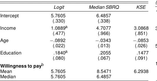
in R$ per month;ageof the family head; and number of years of schooling,education. To facilitate the comparison, all co-variates were centered at the sample means for the model estimation. Table 1 gives coefcient estimates obtained through the censored logit, the Klein and Spady estimator, and the me-dian smoothed binary quantile regression.

Comparison of the coefcient estimates shown in Table 1 re-inforces the claim that all methods provide similar pictures of the center of the willingness-to-pay distribution. Except for the income coefcients, all other estimates are relatively close to one another, with the same sign and basically the same infer-ences. Interestingly, the KSE estimate of the income effect is closer to the median SBRQ than the censored logit estimate. For the remaining coefcients, KSE estimates are closer to cen-sored logit estimates than the median SBRQ.

Table 1. Estimation Results

Logit Median SBRQ KSE

Intercept 5.7605 6.4857 (.330) (.338)

Income 1.0889a 4.7077 3.0868 (.477) (.966) (.851) Age ¡.0892 ¡.0343 ¡.0853 (.022) (.013) (.026) Education .1840a .2055 .1477 (.080) (.067) (.091)

Willingness to payb

Mean 5.7605 8.5471 6.2938 Median 5.7605 6.4857

NOTE: Standard errors are in parentheses.

aSignicant at the 3% level; all other coefcients are signicant at<1% level.

bEstimates are conditional on the sample average of all covariates. The median cannot be computed for the KSE model due to truncation.

A possible explanation for the large difference between the censored logit estimate of the income effect and the semipara-metric models is that the former fails to capture some hetero-geneity structure related to income. Nonetheless, this difference in the income coefcients is very important for welfare analysis based on these models. Even though mean willingness to pay is not signicantly affected, as the similarity of the intercept estimates indicates, signicant differences in welfare measures conditioned on income can be expected.

4.3 Welfare Evaluation

Table 2 lists the estimated proportion of losers for selected costs, according to each model presented in Section 3. Ex-cept for the cost of R$5.76, which corresponds to the mean willingness-to-pay estimate according to the censored logit model, all costs shown in Table 2 were arbitrarily chosen. All estimates were obtained using the methods presented in Sec-tion 3, with¿ ranging from .10 to .70, in .01 increments, for the SBRQ estimates. To ensure monotonicity of the condi-tional quantile functionsx0¯O.¿ /, these functions were smoothed through Ramsay’s (1998) method using the S–PLUS code avail-able at his webpage (www.psych.mcgill.ca/faculty/ramsay.html). This method involves imposing a global monotonicity restric-tion to the optimizarestric-tion problem associated with order-two spline smoothing. Nonetheless, it is important to note that in this application, the effect of imposing monotonicity is negli-gible, because it produces very small changes in the estimated welfare measures.

Each column of Table 2 corresponds to one hypotheticalcost. For each income range there are three lines, corresponding to censored logit (L), KSE estimator (K), and SBRQ (Q). There-fore, for a given estimation method, each cell shows the pro-portion of losers in the total of individualsin that income range. For instance, according to the censored logit model, if the cost is set at R$5.76 per month, then 59.1% of the individuals with a monthly income below R$336 would be worse off. For those with monthly incomes greater than R$2,240, this proportion drops to 30.0%.

Figure 1 shows the proportions of losers for several costs between R$1.00 and R$10.00. The gure indicates that the

Table 2. Proportion of Losers (%)

Income range (R$ per month)

Amount charged (R$ per month) 1.00 3.00 4.50 5.76 7.50 10.00

<336 L 29.3 41.2 50.9 59.1 69.5 81.5 K 30.6 45.6 56.9 63.7 69.2 74.2 Q 22.0 43.7 55.3 56.2 56.9 65.7 336–560 L 23.8 34.6 43.9 52.2 63.3 76.9 K 24.1 34.4 45.9 55.6 64.9 71.5 Q 20.4 33.7 41.7 51.1 55.9 56.6 560–1,120 L 21.1 31.2 40.2 48.3 59.6 74.0 K 22.0 26.9 35.8 45.9 58.6 68.6 Q 20.2 28.4 35.6 38.9 46.0 55.6 1,120–2,240 L 17.9 27.0 35.4 43.3 54.6 69.9 K 23.1 22.1 23.7 28.9 40.9 59.4 Q 19.7 23.7 28.1 34.4 37.4 43.1

>2,240 L 10.9 17.2 23.5 30.0 40.3 56.6 K 19.7 20.4 22.0 23.2 22.4 24.8 Q 17.2 22.2 23.3 24.4 27.4 35.2

NOTE: L, censored logit; K, KSE; Q, SBRQ. At the time of the survey, R$1.15’US$1.

(7)

(a) (b)

(c) (d)

(e)

Figure 1. Proportions of Losers by Income Range: (a) <336; (b) 336–560; (c) 560–1,120; (d) 1,120–2,240; (e)>2,240 (—— SRBQ; ¢ ¢ ¢ ¢ ¢ ¢Logit;¡ ¢ ¡ ¢ ¡KSE).

logit tends to overestimate the proportion of losers, especially when compared with the SBRQ estimates. This overestimation is clearly more accentuated for the income ranges 1,120–2,240 and>2,240. In terms of policy analysis, this overestimation suggests that richer persons may be less affected than the logit approach indicates. If the monthly charge were R$10, for in-stance, then 56.6% of the individuals in the highest income

range would be worse off according to the logit model, whereas this proportion drops to 24.8% for the KSE and 35.2% for the SBRQ.

For the remaining income ranges, the logit curve is relatively close to the KSE curve up to the 55th quantile and to the SBRQ curve up to the 45th quantile. Beyond these quantiles, both the KSE and SBRQ curves have smaller slopes than the logit curve, indicating that the latter places more mass around these quantiles. Because there is a xed amount of mass, this can be interpreted as meaning that the implied willingness-to-pay distribution for both semiparametric approaches is bimodal. In other words, the semiparametric approaches seem to move mass from the center to the upper tail of the distribution.

The apparent bimodality of the willingness-to-pay distribu-tion has important consequences for welfare assessment. In ad-dition to the consequencesfor the estimates of the proportion of losers discussed earlier, bimodality has another important effect on the gains and losses estimates. The reason for this is that moving mass from the center of the distribution to the upper tail is equivalent to increasing the willingness to pay of some indi-viduals (with respect to the logit distribution). As a result, one can expect gains estimates to be larger in the semiparametric approaches. Furthermore, because for most income ranges the differences between implied willingness-to-pay distributions are smaller in the lower tail, as Figure 1 suggests, one can also expect smaller differences in losses than in gains estimates.

Table 3 presents 90% condence intervals associated with the estimated proportions of losers illustrated in Figure 1. To facilitate comparison, all condence intervals were obtained through the same parametric bootstrap procedure. Given the asymptotic normality of the parameter estimates, 1,000 para-meter vectors were drawn from the corresponding multivariate normal distribution for each model. The proportions of losers were computed for each parameter vector, and the condence bounds were dened as the 5th and 95th empirical percentiles of these estimates.

The results reported in Table 3 indicate that the KSE yields smaller condence intervals than the logit in the highest income range. In the remaining income ranges, the KSE produces larger condence intervals than the logit for higher costs and simi-lar intervals at the lower costs. The SBRQ condence intervals

Table 3. Proportions of Losers: 90% Condence Intervals

Amount charged (R$ per month)

1.00 3.00 4.50 5.76 7.50 10.00

<336 L 25.7, 32.7 36.9, 45.1 46.5, 54.9 54.7, 62.9 65.6, 72.8 78.6, 83.8 K 27.5, 36.5 40.1, 48.1 45.8, 59.8 50.4, 65.3 56.4, 71.1 63.5, 78.9 Q 20.2, 25.7 38.5, 50.1 46.8, 55.7 55.3, 56.4 56.8, 57.8 57.9, 70.0 336–560 L 21.1, 26.4 31.2, 37.7 40.2, 47.3 48.3, 55.6 59.6, 66.4 74.0, 79.2 K 21.7, 31.4 33.1, 36.8 40.3, 48.3 44.5, 59.1 50.5, 66.0 59.0, 75.3 Q 18.9, 22.5 32.0, 34.8 38.3, 48.3 43.9, 55.1 53.0, 56.1 56.5, 57.0 560–1,120 L 18.8, 23.5 28.1, 34.2 36.7, 43.5 44.7, 51.8 56.0, 62.9 71.1, 76.6 K 20.5, 28.9 25.2, 32.7 33.3, 38.8 39.1, 49.9 45.6, 62.5 54.1, 70.7 Q 18.4, 21.9 27.3, 28.9 33.6, 36.5 36.9, 40.5 41.9, 54.2 50.8, 56.0 1,120–2,240 L 15.1, 21.1 23.1, 31.2 30.8, 40.2 38.3, 48.3 49.5, 59.6 65.4, 74.0 K 21.0, 27.2 20.7, 28.9 21.9, 32.1 24.3, 38.1 31.0, 51.2 40.7, 64.8 Q 18.1, 21.0 23.3, 24.8 26.9, 29.6 32.0, 35.3 36.0, 38.0 41.1, 50.4

>2,240 L 7.2, 16.6 11.6, 25.2 16.3, 33.3 21.4, 41.0 30.0, 52.3 45.3, 67.9 K 15.8, 25.4 17.4, 25.4 19.8, 26.1 21.2, 27.7 21.1, 31.6 22.3, 45.0 Q 13.2, 20.5 21.6, 22.8 23.1, 24.2 23.9, 26.0 26.1, 30.0 33.1, 35.8

(8)

Table 4. Aggregate Gains and Losses by Income Range (R$ millions per month)

1.00 3.00 4.50 5.76 7.50 10.00

<336 L 5.31,¡.13 3.16,¡.65 1.99,¡1.38 1.28,¡2.28 .64,¡3.96 .21,¡7.18 K 4.86,¡.07 2.69,¡.68 1.61,¡1.58 1.06,¡2.57 .61,¡4.12 .21,¡6.64 Q 5.93,¡.07 3.03,¡.62 1.86,¡1.48 1.42,¡2.16 .86,¡3.11 .11,¡5.21 336–560 L 1.58,¡.02 1.00,¡.11 .66, ¡.23 .44, ¡.40 .23, ¡.73 .08,¡1.41 K 1.46,¡.01 .90,¡.09 .55, ¡.23 .34, ¡.42 .18, ¡.76 .06,¡1.31 Q 2.24,¡.01 1.49,¡.10 1.10, ¡.21 .79, ¡.37 .58, ¡.61 .38, ¡.93 560–1,120 L 1.67,¡.01 1.08,¡.08 .73, ¡.18 .50, ¡.31 .27, ¡.59 .10,¡1.18 K 1.59,¡.01 1.09,¡.06 .71, ¡.14 .45, ¡.26 .22, ¡.53 .07,¡1.03 Q 3.01,¡.01 2.30,¡.07 1.83, ¡.15 1.56, ¡.23 1.18, ¡.40 .78, ¡.75 1,120–2,240 L 1.00,¡.01 .68,¡.03 .47, ¡.07 .33, ¡.13 .19, ¡.25 .07, ¡.52 K .98,¡.01 .77,¡.02 .59, ¡.04 .42, ¡.07 .22, ¡.15 .06, ¡.36 Q 2.09,¡.01 1.76,¡.03 1.50, ¡.05 1.27, ¡.09 1.07, ¡.14 .81, ¡.25

>2,240 L .74,¡.00 .54,¡.01 .41, ¡.02 .31, ¡.03 .20, ¡.06 .09, ¡.16 K .67,¡.00 .54,¡.01 .44, ¡.02 .36, ¡.03 .26, ¡.03 .11, ¡.05 Q 1.74,¡.00 1.51,¡.01 1.40, ¡.02 1.31, ¡.03 1.16, ¡.05 .93, ¡.09

NOTE: Gains are indicated by a positive number losses, by negative numbers. L, censored logit; K, KSE; Q, SBRQ. At the time of the survey, R$1.15’US$1.

are very small in some instances due to discontinuities in the conditional quantile functions. Even though the effect of these discontinuities can probably be eliminated by further smooth-ing, this approach was not considered, because oversmooth-ing would conceal the fact that the quantile models assign very small mass for some costs. In general, apart from obvi-ous cases where this discontinuity effect is present, the widths of the SBRQ condence intervals are in line with those of the logit and the KSE.

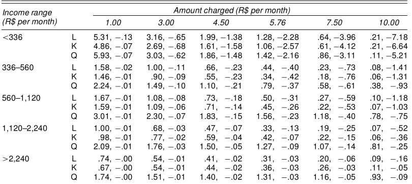
Table 4 presents the estimated gains and losses by income range for the same cost shares considered for the proportion of losers. The number of gainers was obtained by multiplying the proportions represented in Figure 1 by the number of individ-uals in each income range in the population. Aggregate gains were thus obtained by multiplying the number of gainers by the expected gain for each income range.

To facilitate the comparison of results, gains and losses for the logit model were computed as follows. For each income range,F"j_x denoted the logistic distribution with locationxQ0¯O

and scale ¾O, where ¯O and¾O correspond to the estimates ob-tained by maximizing (6). Then willingness-to-pay quantiles were computed usingF¡_"_j_x1.¿ /, with¿ ranging from .01 to .99. Because it is assumed that the project is agood, negative quan-tiles (willingness to pay) should be replaced by 0. Finally, gains and losses were computed using (19) and (20).

The results given in Table 4 reveal that the differences be-tween methods are larger for the gains estimates than for the losses estimates, as discussed earlier, especially when compar-ing the SBRQ and logit estimates. Even though the comparison of the KSE and logit estimates also indicates larger differences in gain estimates than in loss estimates, the effect is diminished by the fact that KSE estimates are clearly downward-biased for the highest income ranges.

The underestimation of gains in the KSE can be easily visu-alized if one notes that the gain estimate dened in Section 3 corresponds to the area to the right of a given cost and above the curves shown in Figure 1. Referring to the income range

>2,240 row in Figure 1, for instance, it is clear that KSE gain estimates should be much larger than the logit’s gain estimates

for any cost share larger than R$4.00. As shown in Table 4, however, the KSE and logit estimates are relatively close to each other.

The downward bias in the KSE’s gains estimates arises from the fact that the estimated probability of a “no” answer for the highest bid value in the sample, R$10.00, is too small at the highest income ranges: 59.4% in the range 1,120–2,240 and 24.8% in the range>2,240. As a result, truncation around R$ 10.00 implies a signicant reduction in the gains estimate.

A similar truncation bias arises in the SBRQ approach when the highest bid value in the sample is too small. The lack of suf-ciently large bids hinders the identication of quantiles far into the upper tail, thus implying some truncation bias. However, in the SBRQ approach, the highest estimable quantile (.7 in this case) is always reached, alleviating the truncation bias. Even though both the KSE and the SBRQ require special attention to bid design, these ndings suggest that the KSE is more sensitive to bid design than the SBRQ.

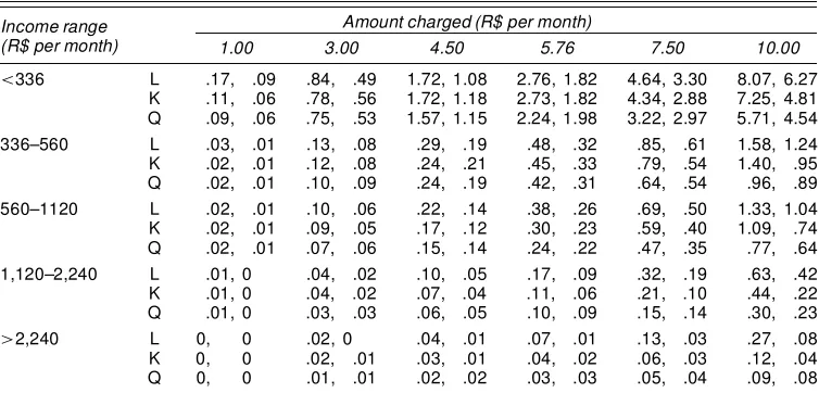
Tables 5 and 6 give the 90% condence intervals obtained through the parametric bootstrap procedure described earlier. These tables show that the condence interval widths relative to the magnitude of the point estimates are more homogeneous than those found for the proportions estimates. This uniformity suggests that the effect of discontinuities of the quantile func-tions is alleviated by the integrationinvolved in the computation of gains and losses.

Unconditional net benet estimates for each cost can be ob-tained by summing gains and losses across income ranges. For a cost share of R$5.76 per month, the net benet according to the logit is¡:29R$ millions per month. Note that because R$5.76 is the mean estimate according to the logit, the net benet is differ-ent from 0 due to an approximation error. In contrast, according to the SBRQ, the net benet for that same cost is R$3.47 mil-lions per month and will be close to 0 (.54) only at a cost of R$7.50 per month. As a result, one can conclude that a project with average cost between 5.76 and 7.50 would have been mistakenly rejected by the compensation criterion had the logit mean estimates been used in the analysis.

It is important noting that the foregoing analysis assumes that the cost share is the same xed amount for all income levels.

(9)

Table 5. Aggregate Gains by Income Range: 90% Condence Intervals (R$ millions per month)

1.00 3.00 4.50 5.76 7.50 10.00

<336 L 4.39, 6.36 2.50, 3.96 1.52, 2.58 .95, 1.71 .46, .90 .14, .31 K 4.46, 5.80 2.41, 3.95 1.40, 2.82 .93, 2.06 .49, 1.22 .14, .42 Q 5.03, 6.75 2.55, 3.62 1.48, 2.36 .96, 1.86 .38, 1.28 0, .49 336–560 L 1.38, 1.81 .84, 1.18 .54, .80 .35, .55 .18, .30 .06, .11 K 1.42, 1.57 .85, 1.11 .50, .82 .30, .61 .16, .37 .04, .12 Q 1.93, 2.57 1.27, 1.73 .91, 1.29 .66, .99 .41, .76 .21, .56 560–1,120 L 1.48, 1.87 .93, 1.26 .61, .87 .41, .61 .22, .34 .08, .13 K 1.55, 1.67 1.02, 1.23 .64, .93 .39, .68 .19, .42 .06, .14 Q 2.57, 3.54 1.93, 2.75 1.51, 2.21 1.25, 1.91 .91, 1.43 .54, 1.07 1,120–2,240 L .85, 1.17 .55, .82 .37, .60 .25, .43 .14, .26 .05, .11 K .91, 1.04 .67, .84 .48, .69 .32, .54 .15, .35 .04, .12 Q 1.81, 2.44 1.49, 2.08 1.25, 1.81 1.05, 1.53 .86, 1.33 .61, 1.04

>2,240 L .53, .96 .36, .76 .25, .61 .18, .49 .10, .35 .04, .18 K .56, .72 .45, .57 .36, .46 .28, .36 .18, .26 .05, .12 Q 1.50, 2.04 1.29, 1.77 1.18, 1.66 1.09, 1.57 .95, 1.41 .76, 1.15

Even though this assumption is justied for simplifying the dis-cussion, we must realize that actual nancing often involves cost shares that are either proportional or progressive. The case where the cost share varies by income range can be easily ac-commodated in the foregoing framework by blocking benet estimates accordingly with the cost share. But if the cost share varies continuously with income, then obtaining exact welfare measures implies considering every point of the income distri-bution, which is clearly not practical. In such cases, a better approach would seem to be to focus on income ranges as an approximation to the exact welfare measure. I am grateful to an anonymous referee for pointing this out.

5. CONCLUSION

This article has presented a comparison of welfare mea-sures in the context of two competing semiparametric models— smoothed binary regression quantiles and the model of Klein and Spady (1993)—and the parametric censored logit. Com-parison of these welfare measures are equivalent to the compar-ison of the implied willingness-to-pay distribution in each of these models.

Results obtained using data from a contingent valuation study for the improvement of water resources in Brazil indicate that estimates at the center of the distribution are very similar regardless of the estimation method used. Moving toward the tails of the benet distribution, the Klein and Spady model’s estimates remain in line with the quantiles approach, whereas the logit seems to fail to capture the heterogeneity struc-ture revealed by the semiparametric approaches. Specically, the Klein and Spady model seems to conrm the bimodality of the willingness-to-pay distribution suggested by the quan-tiles approach.

The apparent bimodality of the willingness-to-pay distri-bution was shown to have important consequences for the computation of gains and losses, yielding different conclu-sions regarding the project’s implementation. According to the Kaldor–Hicks compensation criterion, the project would be unduly rejected for a wide range of average costs if logit es-timates were considered.

A disadvantage of the approach based on the KSE compared with the quantile approach is that its gains estimates seem to be more sensitive to bid design. In the valuation study analyzed in

Table 6. Aggregate Losses by Income Range: 90% Condence Intervals (R$ millions per month)

1.00 3.00 4.50 5.76 7.50 10.00

<336 L .17, .09 .84, .49 1.72, 1.08 2.76, 1.82 4.64, 3.30 8.07, 6.27 K .11, .06 .78, .56 1.72, 1.18 2.73, 1.82 4.34, 2.88 7.25, 4.81 Q .09, .06 .75, .53 1.57, 1.15 2.24, 1.98 3.22, 2.97 5.71, 4.54 336–560 L .03, .01 .13, .08 .29, .19 .48, .32 .85, .61 1.58, 1.24 K .02, .01 .12, .08 .24, .21 .45, .33 .79, .54 1.40, .95 Q .02, .01 .10, .09 .24, .19 .42, .31 .64, .54 .96, .89 560–1120 L .02, .01 .10, .06 .22, .14 .38, .26 .69, .50 1.33, 1.04 K .02, .01 .09, .05 .17, .12 .30, .23 .59, .40 1.09, .74 Q .02, .01 .07, .06 .15, .14 .24, .22 .47, .35 .77, .64 1,120–2,240 L .01, 0 .04, .02 .10, .05 .17, .09 .32, .19 .63, .42 K .01, 0 .04, .02 .07, .04 .11, .06 .21, .10 .44, .22 Q .01, 0 .03, .03 .06, .05 .10, .09 .15, .14 .30, .23

>2,240 L 0, 0 .02, 0 .04, .01 .07, .01 .13, .03 .27, .08 K 0, 0 .02, .01 .03, .01 .04, .02 .06, .03 .12, .04 Q 0, 0 .01, .01 .02, .02 .03, .03 .05, .04 .09, .08

(10)

this article, the highest bid value was too small, leading to sig-nicant underestimation of gains in the highest income ranges.

ACKNOWLEDGMENTS

The author is grateful to two anonymous referees, Milton Barossi, Anil Bera, David Bullock, George Deltas, and espe-cially Roger Koenker for many helpful comments and sug-gestions. The usual disclaimers apply. The S–PLUS code used for estimating the SBRQ was graciously supplied by Gregory Kordas. The author also beneted from the synergy created by the fact that George and Gregory have been work-ing on related methods. Support from CNPq is acknowledged and appreciated.

[Received December 2002. Revised September 2003.]

REFERENCES

Cameron, T. A. (1988), “A New Paradigm for Valuing Non-Market Goods Using Referendum Data: Maximum Likehood Estimation by Censored Lo-gistic Regression,”Journal of Environmental Economics and Management, 15, 355–380.

Chen, H. Z., and Randall, A. (1997), “Semi-Nonparametric Estimation of Bi-nary Response Models With an Application to Natural Resource Valuation,”

Journal of Econometrics, 76, 323–340.

Cosslett, S. R. (1983), “Distribution-Free Maximum Likelihood Estimator of the Binary Choice Model,”Econometrica, 51, 765–782.

(1987), “Efciency Bounds for Distribution-Free Estimators of the Bi-nary Choice and Censored Regression Models,”Econometrica, 55, 765–782. Creel, M., and Loomis, J. (1997), “Semi-Nonparametric Distribution-Free Dichotomous Choice Contingent Valuation,”Journal of Environmental Eco-nomics and Management, 32, 341–358.

Hanemann, W. M. (1989), “Welfare Evaluations in Contingent Valuation Experiments With Discrete Response Data: Reply,”American Journal of Agricultural Economics, 71, 1057–1061.

Horowitz, J. L. (1992), “A Smoothed Maximum Score Estimator for the Binary Response Model,”Econometrica, 60, 505–531.

(1993a), “Semiparametric Estimation of a Work-Trip Choice Model,”

Journal of Econometrics, 58, 49–70.

(1993b), “Semiparametric and Nonparametric Estimation of Quan-tal Response Models,” in Handbook of Econometrics, Vol. 11, eds. G. S. Maddala, C. R. Rao, and H. D. Vinod, New York: Elsevier, pp. 45–84. Klein, R. W., and Spady, R. H. (1993), “An Efcient Semiparametric Estimator

for Binary Response Models,”Econometrica, 61, 387–421.

Koenker, R., and Bassett, G. (1978), “Regression Quantiles,”Econometrica, 46, 33–49.

Kordas, G. (2000), “Binary Regression Quantiles,” unpublished doctoral dis-sertation, University of Illinois, Dept. of Economics.

Li, C. (1996), “Semiparametric Estimation of the Binary Choice Model for Contingent Valuation,”Land Economics, 72, 462–473.

Manski, C. F. (1975), “Maximum Score Estimation of the Stochastic Utility Model of Choice,”Journal of Econometrics, 3, 205–228.

(1986), “Semiparametric Analysis of Binary Response From Sample-Based Samples,”Journal of Econometrics, 31, 31–40.

Mitchell, R. C., and Carson, R. T. (1989),Using Surveys to Value Public Goods: The Contingent Valutation Method, Washington, DC: Resources for the Future.

Ramsay, J. O. (1998), “Estimating Smooth Monotone Functions,”Journal of the Royal Statistical Society, Ser. B, 60, 365–375.