Full Terms & Conditions of access and use can be found at
http://www.tandfonline.com/action/journalInformation?journalCode=ubes20
Download by: [Universitas Maritim Raja Ali Haji] Date: 12 January 2016, At: 23:32
Journal of Business & Economic Statistics
ISSN: 0735-0015 (Print) 1537-2707 (Online) Journal homepage: http://www.tandfonline.com/loi/ubes20
Second-Order Filter Distribution Approximations
for Financial Time Series With Extreme Outliers
J. Q Smith & António A. F Santos
To cite this article: J. Q Smith & António A. F Santos (2006) Second-Order Filter Distribution
Approximations for Financial Time Series With Extreme Outliers, Journal of Business & Economic Statistics, 24:3, 329-337, DOI: 10.1198/073500105000000199
To link to this article: http://dx.doi.org/10.1198/073500105000000199
Published online: 01 Jan 2012.
Submit your article to this journal
Article views: 53
View related articles
Second-Order Filter Distribution Approximations
for Financial Time Series With Extreme Outliers
J. Q. S
MITHDepartment of Statistics, University of Warwick, U.K. (J.Q.Smith@warwick.ac.uk)
António A. F. S
ANTOSFaculty of Economics, Monetary and Financial Research Group (GEMF), University of Coimbra, Portugal (aasantos@fe.uc.pt)
Particle filters are regularly used to obtain the filter distributions associated with state–space financial time series. The most common use today is the auxiliary particle filter (APF) method in conjunction with a first-order Taylor expansion of the log-likelihood. We argue that for series such as stock returns, which exhibit fairly frequent and extreme outliers, filters based on this first-order approximation can easily break down. However, an APF based on the much more rarely used second-order approximation appears to perform well in these circumstances. To detach the issue of algorithm design from problems related to model misspecification and parameter estimation, we demonstrate the lack of robustness of the first-order approximation and the feasibility of a specific second-order approximation using simulated data.
KEY WORDS: Bayesian inference; Importance sampling; Particle filter; State–space model; Stochastic
volatility.
1. INTRODUCTION
One of the two most often reported characteristics associ-ated with financial returns time series is the fat tails in the un-conditional distribution of returns. More observations appear in the tails than for Gaussian processes, giving rise to high kurtosis. The other characteristic is volatility clustering, indi-cating the need to model the variance evolution of the series. Empirical and theoretical investigations have both clearly es-tablished that for short-term financial time series, variances as measures of volatility are time-varying but present some degree of predictability (Bollerslev, Engle, and Nelson 1994; Taylor 1994; Diebold and Lopez 1995; Engle 1995; Campbell, Lo, and MacKinlay 1997; Diebold, Hickman, Inoue, and Schuermann 1998; Ait-Sahalia 1998; Andersen, Bollerslev, and Lange 1999; Christoffersen and Diebold 2000). Variance is used as a mea-sure of risk in a variety of situations, including value-at-risk (VaR) calculations, portfolio allocation, and pricing options.
To model variance dynamics, nonlinear models must be used (Gallant, Rossi, and Tauchen 1993; Hsieh 1993; Bollerslev et al. 1994; Campbell et al. 1997), which in turn requires numerical algorithms for estimation and prediction. The two most com-mon classes of models used in financial time series are the au-toregressive conditional heteroscedastic (ARCH) and stochastic volatility (SV) models. Understanding and predicting the evo-lution of volatility has been a key issue faced by people who must make decisions in financial markets. These two classes of models have been widely used by academics and practitioners. However, new challenges have appeared, and more sophisti-cated algorithms allowing them to deal with real time decisions are needed. Nowadays, data are more and more abundant; one main stream of research uses intraday data, which enable us to take other characteristics of financial time series into ac-count and to measure and estimate other quantities, such as re-alized volatilityandintegrated volatility. Examples of this kind of research have been given by Andersen, Bollerslev, Diebold, and Ebens (2001a), Andersen, Bollerslev, Diebold, and Labys (2001b, 2003), and Andersen, Bollerslev, and Meddahi (2004).
Certainly, taking these new characteristics and measures into account will pose new challenges to the aforementioned mod-els, and the development of well-adapted algorithms, the main objective of this article, is important to the development of mod-els used to characterize financial time series.
For the aforementioned reasons, any state–space model of fi-nancial returns must be nonlinear. The SV model (Taylor 1986) is the simplest nonlinear state–space model. Financial returnsyt are related to unobserved states that are serially correlated. Thus we may write
yt=βexp
α
t 2
εt, εt∼N(0,1), (1) and
αt=φαt−1+σηηt, ηt∼N(0,1), (2) whereαt represents the states of the process for t=1, . . . ,n. Note that the model is characterized by the vector of parame-tersθ=(β, φ, ση). Generalizations of this model can be
con-sidered. In this article we consider the innovation process in the measurement equation to follow a Studenttdistribution.
We assume that the parameters are known or have been previ-ously estimated using, for example, Markov chain Monte Carlo (MCMC) techniques (Jacquier, Polson, and Rossi 1994). Our aim is to present modifications to certain recent particle filter methods to improve predictions in the process defining variance evolution. We adopt a Bayesian state–space approach in which predictions are expressed through the posterior density of states, f(αt|θ,Dt), and the predictive density of returns,f(yt+1|θ,Dt),
rather than through point predictions, whereDt= {y1, . . . ,yt} represents the available information at timet. All densities con-sidered in this article are conditioned by the set of parametersθ,
although later, to simplify notation, we do not make this con-ditioning explicit. The modifications of the more conventional
© 2006 American Statistical Association Journal of Business & Economic Statistics July 2006, Vol. 24, No. 3 DOI 10.1198/073500105000000199
329
330 Journal of Business & Economic Statistics, July 2006
algorithms proposed here are easy to implement, but they never-theless appear to improve the predictive performance of particle filter methods dramatically.
In general, a Bayesian analysis will deliver the posterior den-sity of the state f(αt|θ,Dt)on the unobservable state random variableαt,t=1, . . . ,n. This summarizes all information avail-able at timetrelevant for predicting future values of the series. As new information arrives (e.g.,yt+1), the density of the state
is updated tof(αt+1|θ,Dt+1). This forms the basis of a
recur-sion in which, as new information arrives, at each given time point the state probability densities are sufficient for all predic-tive statements to be updated.
This article focuses on predicting variance evolution in SV models. The method used here is the particle filter as de-veloped by Gordon, Salmond, and Smith (1993), Kong, Liu, and Wong (1994), Fearnhead (1998), Liu and Chen (1998), Carpenter, Clifford, and Fearnhead (1999), de Freitas (1999), Doucet, Godsill, and Andrieu (2000), Doucet, de Freitas, and Gordon (2001), Liu (2001), and Godsill, Doucet, and West (2004). In this method, a distribution that is difficult to analyze algebraically is approximated by a discrete set of points (par-ticles), each with an associated weight. The particles and their associated weights are updated at each time step according to the state dynamics and to take into account the information in the observation. The standard methods for updating the parti-cles are based on importance sampling.
In this article we demonstrate that particle filter algorithms based on a first-order approximation of the log-likelihood, when used with the SV model (1)–(2), can give very unsatis-factory results. We then propose a set of simple extensions to these algorithms that can improve the performance of such fil-ters dramatically. As well as making the filfil-ters more robust, our proposed method greatly simplifies the construction of the filter in comparison with competing algorithms. Our focus here is on the performance of the filter rather than on the estimation of the model. The algorithms that we propose are robust to models that present likelihoods that are not log-concave. This characteristic is missing from the algorithm that serves as a benchmark for this article, the one based on the first-order approximation of the log-likelihood proposed by Pitt and Shephard (1999, 2001). To attempt to isolate the issue of algorithm performance so that it is not confounded with issues related to model misspec-ification and methods used to estimate the parameters, in the empirical section of this article we use two simulated series from two models: the simplest SV model (1)–(2) and its ana-log, which uses Student t innovations, with parameters taken from a well-known source (Jacquier et al. 1994). This enables us to demonstrate that the filter performance issue discussed here is largely independent of model misspecification and para-meter estimation techniques. We can therefore demonstrate that the main issue here is determining the relative efficacy of dif-ferent filters, not primarily because the model is misspecified, but because the more basic particle filter algorithms lack ro-bustness to extreme outliers. Throughout this article we use the term “extreme outlier,” associated with a given series and a run of a particle filter, to describe any observationyt in that series that lies outside the range of particles used to approximate its predictive distribution.
2. FIRST–VERSUS SECOND–ORDER APPROXIMATIONS IN A PARTICLE
FILTER IMPLEMENTATION
Bayes’s rule allows us to assert that the posterior den-sityf(αt|Dt)of states is related to the densityf(αt|Dt−1)prior
Instead of estimating these integrals numerically, particle filter methods approximate these densities using a simulated sam-ple. Particle filters approximate the posterior density of inter-est,f(αt|Dt), through a set ofm“particles”{αt,1, . . . , αt,m}and their respective weights {πt,1, . . . , πt,m}, where πt,j ≥0 and
m
j=1πt,j=1. To implement these filters, we must be able to sample from possibly nonstandard densities. It is possible to de-velop simulation procedures to approximate the distribution of interest and to calculate certain statistics that characterize the distribution. We must be able to implement these procedures sequentially as states evolve over time and new information be-comes available. This implementation needs to be efficient, and the approximations need to remain good as we move through the sequence of states.
From a sequential perspective, the main aim is to update the particles att−1 and their respective weights,{αt−1,1, . . . ,
αt−1,m}and {πt−1,1, . . . , πt−1,m}. These are the particles and respective weights that approximate a given density, usually a continuous density function. In this context, the target density is often hard to sample from, so we must use an approximating density. We can sample using this density and then resample as a way of approximating better the target density. This is the procedure associated with the sampling importance resampling (SIR) algorithm. However, Pitt and Shephard (1999, 2001) pointed out that using f(αt|αt−1)as a density approximating
f(αt|Dt)is not generally efficient because it constitutes ablind proposal that does not take into account the information con-tained in yt. To improve efficiency, we include this informa-tion in the approximating density. The nonlinear/non-Gaussian component of the measurement equation then starts to play an important role, and certain algebraic manipulations need to be carried out to use standard approximations. This can be accom-plished by sampling from a higher-dimensional density. First, an indexkis sampled, which defines the particles att−1 that are propagated tot, thus defining what Pitt and Shephard called an auxiliary particle filter. This corresponds to sampling from
f(αt,k|Dt)∝f(yt|αt)f(αt|αt−1)πk, k=1, . . . ,m, (5) where πk represents the weight given to each particle. We can sample first from f(k|Dt) and then from f(αt|k,Dt), ob-taining the sample{(αt,j,kj);j=1, . . . ,m}. The marginal den-sityf(αt|Dt)is obtained by dropping the indexk. If information contained inyt is included, then this resolves the problem of too many states with negligible weight being carried forward, thereby improving numerical approximations. Now the target
distribution becomesf(αt,k|Dt)and the information inytis car-ried forward byπk. The next step is to define a density approx-imatingf(αt,k|Dt). One of the simplest approaches, described by Pitt and Shephard (1999, 2001), is to define
f(αt,k|Dt)≃g(αt,k|Dt)∝f(yt|µt,k)f(αt|αt−1)πk, (6) whereµt,k is the mean, the mode, or a highly probable value associated withf(αt|αt−1).
Outliers are commonly observed in financial series, and for such datum the information in the prior is very different from that contained in the likelihood. This means that only very few particles used to approximate the filter density att−1 are prop-agated to approximate the filter density att. This gives rise to sample impoverishment.
Let g(·|·) represent any density approximating the target density f(·|·). If the likelihood is log-concave, with a first-order approximation, then it can be easily ascertained that g(yt|αt, µt,k)≥f(yt|αt)for all values ofαt, whereg(yt|αt, µt,k) constitutes the first-order approximation off(yt|αt)aroundµt,k.
This means that with the approximating density, in this context we can define a perfect envelope for the target density, and a rejection sampler can be implemented (see Pitt and Shephard 1999, 2001). But we can demonstrate here that this algorithm is not robust to extreme observations when the aim is to update the filter density within the model (1)–(2). We need a better approximation of the likelihood function to define the required approximating density.
The main modification considered is the definition of a second-order (instead of a first-order) approximation that is taken around a different pointα∗t from that proposed by Pitt and Shephard (1999, 2001). The details of the algebra applied to the model used in this article are given later, but in general we are defining a second-order approximation aroundαt∗for the log-likelihood, logf(yt|αt)=l(αt), which we designate as Because we propose using a second-order approximation, we cannot guarantee that the approximating density constitutes an envelope to the target density, as we can with the first-order approximation, and we need to specify the algebra to im-plement the sampling importance resampling algorithm. This algebra depends on the point used to perform the Taylor expan-sion of the log-likelihood. Pitt and Shephard (1999, 2001) used
αt∗=φαt−1 and suggested other possible points, such as the
mode of the posterior distribution or a point between the pos-terior and prior modes. Here our main concern is to choose an expansion point to, as much as possible, avoid a given filter de-generating, as happens, for example, when a distribution with a continuous support is approximated by a single point.
A second-order approximation defines a Gaussian approxi-mating density, and the variance of the approxiapproxi-mating density is defined through the second derivative of the log-likelihood. When the likelihood is not log-concave, it is not always possi-ble to define meaningful Gaussian approximations for all pos-sible points considered. To overcome this problem, and also
to obtain a less complicated algebra, we consider a second-order approximation around the point that maximizes the log-likelihood. Assuming the regularity conditions that guarantee that the likelihood has a maximum, we letα∗t denote the point that maximizes the log-likelihood, and we havel′(αt∗)=0. In
which resembles the log-kernel of a Gaussian density with meanαt∗and variance−1/l′′(α∗t). When applied to the model in (1)–(2), we find that it simplifies the algebra considerably, and, because we are assuming that the log-likelihood has a maxi-mum, we havel′′(αt∗) <0, thus defining a meaningful Gaussian approximation. The componentl(αt∗)is absorbed into the nor-malizing constant, and the remainder is the log-kernel of a Gaussian density. Then we needl′′(αt∗) <0, because−1/l′′(αt∗)
defines the variance of the corresponding distribution.
In this article we claim that the particle filter algorithm im-plemented by Pitt and Shephard (1999, 2001), based on a first-order approximation of the likelihood function, is not robust to extreme outliers. We demonstrate, however, that a second-order approximation (suggested but not implemented by these au-thors), used in conjunction with an appropriate expansion point, gives meaningful results supported by straightforward algebra. The calculation of appropriate formulas is presented in the next section. The algebra for specifying the first-order filter was cal-culated by Pitt and Shephard (1999, 2001), and the algebra for the second-order filter using a generic pointµt,kis given in the Appendix.
3. APPROXIMATIONS BASED ON MAXIMUM LIKELIHOOD POINTS
For likelihoods associated with extreme outliers and the usual classes of SV models, it can be shown theoretically that the ex-pansion pointµt,k=φαt−1,k, suggested by Pitt and Shephard
(1999, 2001), is not where we should expect the posterior den-sity to center its weight (Dawid 1973). For the class of sto-chastic volatility models, the weight should be more closely centered around the maximum of the likelihood function. In a standard SV model, calculation of this quantity is straightfor-ward, and we find that
α∗t =log
Therefore, we propose using the Taylor series approximation defined in (7) withα∗t as here. There are two main advantages to using this approximation. First, the algebra needed to imple-ment the algorithm is greatly simplified; second, this procedure can be extended to include the cases where the likelihood is no longer strictly log-concave. Here we focus on the first ad-vantage. The algebra is simpler because we are combining the log-kernel of two Gaussian densities, one given by the transi-tion density and the other given by12l′′(αt∗)(αt−αt∗)2, which is the log-kernel of a Gaussian density with meanαt∗and variance −1/l′′(α∗t)=2.
In this setting, we need to take into account the first-stage weights, those that define which particles approximating the fil-ter density att−1 will be carried forward to define the filter
332 Journal of Business & Economic Statistics, July 2006
density att. Using the notation of (5), these are denoted byπk and carry the information contained inyt. The second-order ap-proximation of the log-likelihood combined with the log-prior gives an approximating density The particles at t−1 that are used to define the approximat-ing density are sampled usapproximat-ing first-stage weights, now defined through (11), which depend on the information inytasα∗t de-pends on yt. When sampling the index k from a distribution proportional to (11), the particleαt−1,k is chosen, and the den-sity, assuming the role of prior denden-sity, assumes a Gaussian form with meanµt,k=φαt−1,kand variance ση2. This is
com-bined with a Gaussian density with mean αt∗ and variance −1/l′′(αt∗)=2. After the particles have been sampled, they must be resampled to take into account the target density. They are resampled using the second-stage weights
logwj= − After the resampling stage, an approximation of the target pos-terior distribution of the states attis available; this is used as a prior distribution to update the states att+1, and the process continues recursively as new information arrives.
To summarize, the particles att−1 propagated to update the distribution of the states attare chosen randomly according to the weights defined by (11). These weights are influenced by the information contained in yt. By conditioning on each par-ticle chosen through the first-stage weights, new parpar-ticles are sampled. Because these come from an approximating distribu-tion, a second step is needed. The particles are resampled using the weights defined by (15)–(16). Our modification, outlined earlier, makes this second-order auxiliary particle filter (APF) straightforward and quick to implement.
4. A MODEL EXTENSION
It has long been known that there are better models than the standard SV model for financial returns series. Two of the best
known modifications of the SV model use Studenttinstead of Gaussian innovations and allow for the possibility of leverage effects. Consider then that the innovation process in (1) follows a scaled Studenttdistribution withυdegrees of freedom,
εt∼
υ−2
υ tυ. (17)
Second-order approximations around the proposed point in the preceding section allow us to produce results analogous to (9)–(16), and the choice of the expansion point greatly simpli-fies calculations in this case. Now the point used to perform the approximation is different, and the second derivative of the log-likelihood function, used to define the variance of the ap-proximating distribution, is also different.
The foregoing algorithms can be extended quite straight-forwardly by defining the new approximation for the log-likelihood function. In this case, the log-log-likelihood can be written as The first derivative is given by
l′(αt)=
υy2t −(υ−2)β2exp(αt) 2(υ−2)β2exp(αt)+2y2t
, (19) and the second derivative is
l′′(αt)= −
(υ2−υ−2)β2exp(αt)y2t 2((υ−2)β2exp(α
t)+y2t)2
<0. (20) Using these results, we can easily define the value of αt that maximizes the likelihood function. Solving the equation l′(αt)=0, we obtain all values ofαt. The other component that must be calculated is the value of the second derivative on the point that maximizes the log-likelihood. It is straightforward to show that
s2t = − 1 l′′(α∗
t)
=2+2
υ. (22)
In this context, (11) is reformulated, and we obtain
g(yt|αt∗)=exp follows. The analog for the density defined in (12) is still a Gaussian density function, but nowµ∗t,kandσt2,kare defined as
After the approximating draws are obtained, αt,j, for j =
1, . . . ,m, the resampling step is performed using the weights logwj= −
αt,j
2 −
υ+1 2 log
1+ y
2
t
(υ−2)β2exp(α
t,j)
+υ(αt,j−α
∗
t)2 4υ+4 (26) and
πt,j= wj
m i=1wi
, j=1, . . . ,m. (27) With the Studenttextension, implementation of the algorithm is still uncomplicated, because, as in the previous case, we have a likelihood that is log-concave and a maximum that can be calculated analytically.
5. AN EMPIRICAL DEMONSTRATION
To demonstrate the efficiency of our second-order filter over its first-order competitors, independent of estimation consid-erations, we first analyzed a set of simulated series using the correct filter, then compared filters known to be misspecified. We simulated series from two different models, the standard SV model and the SV model with Studenttinnovations. We used the parameters obtained by Jaquier et al. (1994) as the estimates of the parameters associated with IBM and TEXACO stocks. The parameters, translated to the parameterization used in this article, are given in Table 1. We chose these two stocks be-cause one seems to exhibit a lower degree of persistence (IBM) and the other seems to have a higher degree of persistence (TEXACO). We simulated 1,000 observations for each stock using the standard SV model, and also performed simulations
Table 1. Simulation Parameters
Parameters IBM TEXACO
β 2.9322 2.2371
φ .83 .95
ση .4 .23
NOTE: This table gives the values of the parameters used to simulate the four series used in this section. These parameters are translated from Jaquier et al. (1994) as the authors used another parameterization.
for the same parameters, but assuming that the innovations fol-lowed a scaled Studenttdistribution with 5 degrees of freedom. We then applied the filters to the four series using the correct model specification. We also ran simulations in which the filter design for the Gaussian distribution was applied to the Studentt distribution and vice versa. Of course, in this case we obtained poor approximations compared with those obtained using the correct filter, although the main point is still relevant—that us-ing the first-order approximation, we can get extreme sample impoverishment.
From these series, depicted in Figure 1, we can see two of the essential characteristics commonly found in any real data financial time series, that is, volatility clustering and extreme observations, which can be modeled by a process that allow time-varying variances with persistence and unconditional dis-tribution with fat tails. The information contained in the ex-treme observations seen in these series and models cannot be dealt with effectively using standard first-order approximations within an APF.
We ran the filters, using first- and second-order approxima-tions, for the two simulated series obtained through a standard SV model, and we found that one filter distribution that could not be approximated properly for TEXACO, and nine for IBM. This is due to the fact that these observations assume extreme
Figure 1. Simulated Data Using the Parameters of Table 1. The left side series are obtained assuming the model in (1)–(2). When we consider Student t innovations another parameter is added, the parameterυ, which represents the degrees of freedom. Here we useυ=5, and in this way we simulated the series on the right side.
334 Journal of Business & Economic Statistics, July 2006
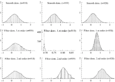
Figure 2. Density Estimation Comparison for TEXACO for Reference Observation 919. The first row shows the approximating smooth densities for this observation, as well for its predecessor and its successor. The second row gives the approximating filter densities obtained through a first-order particle filter, and the third row gives the approximating filter densities using the second-order particle filter.
values for which the first-order filter cannot accommodate the information contained in them.
Figures 2 and 3 depict smoothing and then filtered state den-sity approximations around two potentially problematic obser-vations for the filters, the first to appear in each series, the 919th for TEXACO and the 24th for IBM. The first row presents the smoothing densities of the states. These provide a rough benchmark for the true distribution of the state, although they are obtained by conditioning in a different information set, so they simply give an indication of the type of distribution we might expect to see, albeit with some shift in the mean and vari-ance. We obtained the approximating smoothing densities using MCMC simulation techniques. It is clear that when we applied the first-order filter to update the information contained in the problematic observations, we obtained meaningless results. The density function in a given range, which we know from theoret-ical considerations must be continuous, was approximated by a small number of distinct particles and in extreme cases by a single particle. But this problem clearly did not emerge when we applied a second-order filter to approximate the densities. In the second row of Figures 2 and 3, the filter densities as-sociated with the information in the problematic observations were obtained using the first-order approximation. To make the comparisons clearer, we also present the respective densities for the preceding and succeeding observations of those considered problematic. The densities based on the second-order approx-imation can be compared with these and the smoothing densi-ties, and in this case they exhibit a more sensible configuration. When a model is misspecified, the forecasts obviously be-come worse. We ran the filter based on a standard SV model
for a dataset obtained from a model with Studenttinnovations. As might be expected, the Studentt distribution produces se-ries with more extreme observations. When we used the filter assuming Gaussian innovations, due to model misspecification, we obtained significantly worse results than when we used the true model for all filters and their associated approximations.
However, the first-order approximation gave far more de-generacy when we applied the filter based on a model with Gaussian innovations to a model in which the true innovations are Studentt. When using the first-order filter without the mis-specification of the model, we had one problematic observa-tions for TEXACO and nine problematic observaobserva-tions for IBM. When we applied the filter to the series with Student t inno-vations, we found 5 observations for TEXACO and 16 ob-servations for IBM in which the filter could not update the information. In contrast, although the second-order filter suming Gaussian innovations gave worse results than that as-suming the true Studentt predictions, we did not experience the degenerate breakdown apparent for the first-order filter.
Figure 4 compares the performance of the filters empirically by showing first- and second-order filter Gaussian approxima-tions and second-order filter Studenttapproximations for two typical extreme observations. Note that the errors associated with model misspecification are of a smaller order than those associated with the failure of the filter approximation. These results are entirely representative of other comparisons that we made.
To demonstrate even further the lack of robustness of a par-ticle filter based on a first-order approximation, we again used the IBM series based on the standard SV model, and for the first
Figure 3. Density Estimation Comparison for IBM for Reference Observation 24. The first row shows the approximating smooth densities for this observation, as well its predecessor and its successor. The second row presents the approximating filter densities obtained through a first-order particle filter, and the third row gives the approximating filter densities using the second-order particle filter.
Figure 4. Filter Densities Associated With the Distribution of the States at Observation 79 for IBM and 128 for TEXACO, Simulated Through an SV Model With Student t Innovations. The first row represents the filter applied without model misspecification, whereas the second and third rows are from a filter assuming Gaussian innovations, the second row using a second-order filter, and the third row using a first-order filter.
336 Journal of Business & Economic Statistics, July 2006
Table 2. First-Order versus Second-Order Filter Comparison
Statistic E(ˆ α24|D24)f E(ˆ α24|D24)s
Mean .7651 .8077
Standard deviation .2477 .0172
Coefficient of variation .3238 .0213
Minimum −.6649 .7626
Maximum 1.9847 .8908
NOTE: This table presents the summary of statistics from a simulation where the distribution of the mean estimates of the states associated with the 24th observations in the IBM stock are calculated. The estimates of the first-order filter, designated by the subscript “f,” and the second-order filter, with the subscript “s,” are compared.
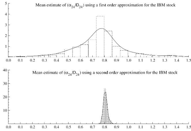
extreme observation (the 24th) approximated the distribution of the estimate to the mean of the state in the corresponding obser-vation. The estimated mean is sometimes obtained using only a small number of particles, and, as has been demonstrated by, for example, Liu and Chen (1998) and Pitt and Shephard (1999), as we use less even weights, the variance of our estimates tends to increase.
The second-order particle filter performed considerably bet-ter than the first-order filbet-ter. In the simulation the filbet-ters were run 1,000 times, and the estimated mean of the filter distribution at observation 24 was recorded. Table 2 gives the descriptive statistics associated with the two approximating distributions, which are also depicted in Figure 5. The estimated means of the state mean did not differ much. However, a much greater uncer-tainty was associated with the estimate yielded by the first-order filter. Because of parameter and model uncertainty, we are usu-ally more interested in the approximation of an entire density than just a simple statistic. Then, although we can sometimes obtain a sensible value for the estimated mean for the filter dis-tribution of the state, most of the time this estimate is based on a very small number of distinct values. For example, in the extreme case of sample impoverishment, the mean can be ob-tained using just a single particle. The estimate based on the first-order filter can give very imprecise results. Using the re-sults in Table 2, we can see that in this simulation the coefficient
of variation was reduced by more than 90% when we used the second-order filter instead of the first-order filter, as we might have expected.
6. CONCLUSION
We have demonstrated that it is possible to develop APFs based on a second-order Taylor series approximation, which, unlike their first-order analog, perform well for series with ex-treme observations, which are fairly common in financial time series. We are currently developing analogous procedures for time series whose likelihood is not log-concave. Our prelimi-nary results are encouraging and will be presented in a future article.
ACKNOWLEDGMENTS
The authors thank the editor, associate editor, and anonymous referees for their valuable comments.
APPENDIX: SECOND–ORDER APPROXIMATION BASED ON THE PRIOR MEAN
Using the points used by Pitt and Shephard (1999, 2001) to define the first-order filter,µt,k=φαt−1,k, we present the
al-gebra associated with the second-order filter. In this case, apart from the formulas, the main difference is that only the sampling importance resampling algorithm can be used. The approxima-tion g(yt|αt, µt,k)is defined through the second-order Taylor approximation of logf(yt|αt)aroundµt,k,
logg(yt|αt, µt,k)
∝l(µt,k)+l′(µt,k)(αt−µt,k)+ 1 2l
′′(µ
t,k)(αt−µt,k)2 =const−αt
2 −
y2tAt,k 2β2exp(µ
t,k)
,
Figure 5. The Approximating Densities Associated With the Mean Estimate of the States at Observation 24 for IBM, Using the Standard SV Model. The first was obtained using the first-order filter; the second, using the second-order filter.
where
At,k=(αt−µt,k)+
(αt−µt,k)2
2 −1.
Using this second-order approximation, the density g(αt, k|Dt)is factorized in the elements in it must be resampled to obtain a sample that gives a better approximation of the target densityf(αt,k|Dt). The weights used in this resampling step are
logwj= − y
These are the so-called “second-stage” weights that allow mod-ification of the approximating distribution toward the target dis-tribution. Obviously, these weights must be distributed more evenly than those from the first-order approximation, because the second-order approximation allows a better approximation of the target distribution.
[Received August 2003. Revised August 2005.]
REFERENCES
Ait-Sahalia, Y. (1998), “Dynamic Equilibrium and Volatility in Financial Asset
Markets,”Journal of Econometrics, 84, 93–127.
Andersen, T. G., Bollerslev, T., Diebold, F. X., and Ebens, H. (2001a), “The
Dis-tribution of Realized Stock Return Volatility,”Journal of Financial
Eco-nomics, 61, 43–76.
Andersen, T. G., Bollerslev, T., Diebold, F. X., and Labys, P. (2001b), “The
Dis-tribution of Exchange Rate Volatility,”Journal of the American Statistical
Association, 96, 42–55.
(2003), “Modeling and Forecasting Realized Volatility,”
Economet-rica, 71, 579–625.
Andersen, T. G., Bollerslev, T., and Lange, S. (1999), “Forecasting Financial
Market Volatility: Sample Frequency vis-á-vis Forecast Horizon,”Journal of
Empirical Finance, 6, 457–477.
Andersen, T. G., Bollerslev, T., and Meddahi, N. (2004), “Analytic Evaluation
of Volatility Forecasts,”International Economic Review, 45, 1079–1110.
Bollerslev, T., Engle, R. F., and Nelson, D. (1994), “ARCH Models,” in
Hand-book of Econometrics, Vol. 4, eds. R. Engle and D. McFadden, Amsterdam: Elsevier, pp. 2959–3038.
Campbell, J. Y., Lo, A. W., and MacKinlay, C. (1997),The Econometrics of
Financial Markets, Princeton, NJ: Princeton University Press.
Carpenter, J., Clifford, P., and Fearnhead, P. (1999), “An Improved Filter for
Non-Linear Problems,”IEE Proceedings in Radar, Sonar Navigation, 146,
2–7.
Christoffersen, P. F., and Diebold, F. X. (2000), “How Relevant Is Volatility
Forecasting for Financial Risk Management?”The Review of Economic and
Statistics, 82, 12–22.
Dawid, A. P. (1973), “Posterior Means for Large Observations,”Biometrika,
60, 664–666.
de Freitas, J. F. G. (1999), “Bayesian Methods for Neural Networks,” unpub-lished doctoral thesis, University of Cambridge, Engineering Dept. Diebold, F. X., Hickman, A., Inoue, A., and Schuermann, T. (1998), “Scale
Models,”Risk, 11, 104–107.
Diebold, F. X., and Lopez, J. A. (1995), “Modeling Volatility Dynamics,” in
Macroeconomics: Developments, Tensions, and Prospects, ed. K. Hoover, Boston: Kluwer Academic, pp. 427–472.
Doucet, A., Godsill, S., and Andrieu, C. (2000), “On Sequential
Simulation-Based Methods for Bayesian Filtering,” Statistics and Computing, 10,
197–208.
Doucet, A., de Freitas, N., and Gordon, N. (2001),Sequential Monte Carlo
Methods in Practice, New York: Springer-Verlag.
Engle, R. F. (1995),ARCH: Selected Readings, Oxford, U.K.: Oxford
Univer-sity Press.
Fearnhead, P. (1998), “Sequential Monte Carlo Methods in Filter Theory,” un-published doctoral thesis, Merton College, University of Oxford.
Gallant, A. R., Rossi, P. E., and Tauchen, G. (1993), “Nonlinear Dynamics
Structures,”Econometrica, 61, 871–907.
Godsill, S. J., Doucet, A., and West, M. (2004), “Monte Carlo Smoothing for
Non-Linear Time Series,”Journal of the American Statistical Association,
99, 156–168.
Gordon, N. J., Salmond, D. J., and Smith, A. F. M. (1993), “A Novel Approach
to Non-Linear and Non-Gaussian Bayesian State Estimation,”IEE
Proceed-ings F, 140, 107–113.
Hsieh, D. A. (1993), “Implications of Nonlinear Dynamics for Financial Risk
Management,”Journal of Financial and Quantitative Analysis, 28, 41–64.
Jacquier, E., Polson, N. G., and Rossi, P. E. (1994), “Bayesian Analysis of
Sto-chastic Volatility Models,”Journal of Business & Economic Statistics, 12,
371–417.
Kong, A., Liu, J. S., and Wong, W. H. (1994), “Sequential Imputations and
Bayesian Missing-Data Problems,”Journal of the American Statistical
Asso-ciation, 89, 278–288.
Liu, J. S. (2001),Monte Carlo Strategies in Scientific Computing, New York:
Springer-Verlag.
Liu, J. S., and Chen, R. (1998), “Sequential Monte Carlo Methods for Dynamic
Systems,”Journal of the American Statistical Association, 93, 1032–1044.
Pitt, M. K., and Shephard, N. (1999), “Filtering via Simulation: Auxiliary
Par-ticle Filters,”Journal of the American Statistical Association, 94, 590–599.
(2001), “Auxiliary Variable–Based Particle Filters,” in Sequential
Monte Carlo Methods in Practice, eds. A. Doucet, J. F. G. de Freitas, and N. J. Gordon, New York: Springer-Verlag, pp. 273–293.
Taylor, S. J. (1986),Modelling Financial Time Series, Chichester, U.K.: Wiley.
(1994), “Modelling Stochastic Volatility: A Review and Comparative
Study,”Mathematical Finance, 4, 183–204.