Full Terms & Conditions of access and use can be found at
http://www.tandfonline.com/action/journalInformation?journalCode=ubes20
Download by: [Universitas Maritim Raja Ali Haji] Date: 12 January 2016, At: 23:03
Journal of Business & Economic Statistics
ISSN: 0735-0015 (Print) 1537-2707 (Online) Journal homepage: http://www.tandfonline.com/loi/ubes20
Modeling Around-the-Clock Price Discovery for
Cross-Listed Stocks Using State Space Methods
Albert J Menkveld, Siem Jan Koopman & André Lucas
To cite this article: Albert J Menkveld, Siem Jan Koopman & André Lucas (2007) Modeling
Around-the-Clock Price Discovery for Cross-Listed Stocks Using State Space Methods, Journal of Business & Economic Statistics, 25:2, 213-225, DOI: 10.1198/073500106000000594
To link to this article: http://dx.doi.org/10.1198/073500106000000594
Published online: 01 Jan 2012.
Submit your article to this journal
Article views: 178
View related articles
Modeling Around-the-Clock Price Discovery for
Cross-Listed Stocks Using State Space Methods
Albert J. M
ENKVELDDepartment of Finance, Vrije Universiteit, Amsterdam, The Netherlands, NL-1081HV (ajmenkveld@feweb.vu.nl)
Siem Jan K
OOPMANDepartment of Econometrics and Tinbergen Institute, Vrije Universiteit, Amsterdam, The Netherlands, NL-1081HV (s.j.koopman@feweb.vu.nl)
André L
UCASDepartment of Finance and Tinbergen Institute, Vrije Universiteit, Amsterdam, The Netherlands, NL-1081HV (alucas@feweb.vu.nl)
U.S. trading in non-U.S. stocks has grown dramatically. Around the clock, these stocks trade in the home market, in the U.S. market, and, potentially, in both markets simultaneously. We develop a general method-ology based on a state space model to study 24-hour price discovery in a multiple-markets setting. As opposed to the standard variance ratio approach, this model deals naturally with (1) simultaneous quotes in an overlap, (2) missing observations in a nonoverlap, (3) noise due to transitory microstructure ef-fects, and (4) contemporaneous correlation in returns due to market-wide factors. We apply our model to Dutch stocks, cross-listed in the United States. Our findings suggest a minor role for the New York Stock Exchange in price discovery for Dutch shares, in spite of its nontrivial and growing market share. KEY WORDS: Efficient price; Financial markets; High-frequency data; Kalman filter; Unobserved
components time series models.
1. INTRODUCTION
In the last decade, international firms have increasingly sought a U.S. listing, oftentimes achieved through cross-listing their shares on either the New York Stock Exchange (NYSE) or the NASDAQ. At the end of 2002, 467 non-U.S. firms were listed on the NYSE and generated approximately 10% of total volume that year (numbers are taken from the 2003 annual re-port). The NASDAQ lists even more non-U.S. firms. This trend has prompted many academic studies. Most of them focus on the benefits of cross-listing, such as reduced cost of capital and enhanced liquidity of a firm’s stock (see Karolyi 2006 for a survey).
A relatively unexplored question is how much U.S. trading contributes to around-the-clock price discovery over and above domestic trading. Reasoning could go both ways. On the one hand, the home market, being closest to where the information is produced, may be most important (see, e.g., Solnik 1996; Hau 2001; Bacidore and Sofianos 2002). On the other hand, U.S. stock exchanges, being the largest and most liquid exchanges in the world, may also play an important role in price discovery for non-U.S. stocks, particularly now that their share in total U.S. volume is rapidly increasing. Chan, Hameed, and Lau (2003), for example, found that trading location matters irrespective of business location for a group of companies that changed their listings from Hong Kong to Singapore. The evidence for Cana-dian stocks and, if we focus on the overlapping period only, for Dutch, German, and Spanish stocks shows that the NYSE contributes significantly less to price discovery than the do-mestic exchange (see Eun and Sabherwal 2003; Hupperets and Menkveld 2002; Grammig, Melvin, and Schlag 2005a; Pascual, Pascual-Fuste, and Climent 2001, respectively). Grammig et al. (2005b) documented, based on a cross-section of Canadian,
British, French, and German stocks, that the NYSE contribution increases in its liquidity relative to that of the home market.
Our objective is to develop a general methodology to de-termine how informative trading is for around-the-clock price discovery in a multiple-markets setting. It enables the analysis of the questions raised for U.S. trading in non-U.S. stocks but applies more generally to securities trading in multiple venues and, possibly, multiple time zones. Examples include securities trading on multiple trading platforms or through multiple bro-ker/dealers, oftentimes referred to as fragmented trading (see Stoll 2001a), London and Tokyo trading in U.S. treasury secu-rities (see, e.g., Fleming and Lopez 2003), and foreign listings on European exchanges (see Pagano, Randl, Roëll, and Zechner 2001).
The empirical literature on around-the-clock price discov-ery dates back tosingle-market studies comparing variance ra-tios of open-to-close and close-to-open returns. They generally found that trading periods produce more information than non-trading periods (see Oldfield and Rogalski 1980; French and Roll 1986; Harvey and Huang 1991; Jones, Kaul, and Lipson 1994). Chan, Fong, Kho, and Stulz (1996), for example, used variance ratios to study U.S. trading in European stocks and found that the morning-to-afternoon variance ratio is signif-icantly larger than a benchmark ratio based on U.S. control stocks. A natural extension of variance ratios to our multiple-markets setting is to fix time points in the day, calculate the vari-ance of intraday returns, take a cross-sectional average (across stocks), and study the intraday pattern. This approach could fail
© 2007 American Statistical Association Journal of Business & Economic Statistics April 2007, Vol. 25, No. 2 DOI 10.1198/073500106000000594
213
for three reasons. First, in our setting, calculating returns in-volves arbitrary choices for prices in overlapping periods, as we observe prices in multiple markets. Second, midquotes and transaction prices are potentially noisy proxies for the unob-served efficient price as a result of microstructure effects, due to, for example, market making or a nonzero tick size (see, e.g., Stoll 2001b). These transitory effects, or “noise,” are negligi-ble for weekly, monthly, or annual returns, but not for intraday returns. This is illustrated by studies that find 24-hour returns based on opening prices to be, on average, up to 20% more volatile than those based on closing prices (see Amihud and Mendelson 1987; Stoll and Whaley 1990; Gerety and Mulherin 1994; Forster and George 1996). Transitory effects are poten-tially distorting as they artificially inflate price discovery within a trading day. Third, Ronen (1997, p. 184) criticized “many of the intradaily variance ratios used in this literature” because sta-tistical inference ignores cross-sectional correlation in returns.
In this article we develop a methodology based on a state space model to account for the three criticisms of the standard variance ratio approach. Such a model arises naturally after characterizing the (unobserved) efficient price process as a ran-dom walk (see, e.g., Campbell, Lo, and MacKinlay 1997). To study around-the-clock price discovery, we endow this random walk with deterministic, time-varying volatility. To account for transitory price changes, we model the observed midquote as the unobserved efficient price plus temporary deviations due to “microstructure” effects and short-term market under- or overreaction to information (see, e.g., Amihud and Mendelson 1987). In the overlap, both midquotes are functions of the same unobserved efficient price plus idiosyncratic temporary devia-tions. To account for cross-correlation in returns, we model re-turns as the sum of a common and an idiosyncratic factor, where the common factor captures, for example, macroeconomic in-formation or portfolio-wide liquidity shocks. The model is esti-mated using maximum likelihood. The Kalman filter is used to calculate the likelihood at each step in the optimization. A ma-jor advantage of the Kalman filter in our setting is that it deals naturally with missing values in the nonoverlap trading peri-ods. Moreover, it allows for decomposition of an observed price change into a transitory and a permanent component based on the entire sample (see Durbin and Koopman 2001).
For partially overlapping markets, the state space approach compares favorably to alternative methodologies. In related work, Hasbrouck (1995) proposed a vector error correction model to measure “information shares” of exchanges for price discovery during the period when both exchanges are open. Although this approach accounts for transitory price changes, it does not extend to our setting, because it cannot deal with missing values in one of the markets in the nonoverlap. A gen-eralized state space approach, on the other hand, does nest the Hasbrouck model. We will come back to this issue when discussing the model. Barclay and Hendershott (2003) used weighted price contributions (WPCs) to study how informative after-hours trading is. The WPC approach, however, does not explicitly allow for transitory effects. In their pioneering study, Barclay and Warner (1993, p. 300) developed WPCs and ac-knowledged that “it is not clear how any bias from ignoring temporary price-change components could drive our results.”
The state space model is estimated based on a 1997–1998 sample of Dutch blue chips cross-listed in New York. The
United Kingdom excluded, Dutch stocks are the European stocks that generate the most volume in New York. The dataset is rich, because it includes all trades and quotes on both sides of the Atlantic, as well as intraday quotes on the exchange rate and intraday prices on the major Dutch index and the Standard & Poor’s (S&P) 500.
The results demonstrate the empirical relevance of the model, because the estimated variance pattern of the efficient price in-novations differs significantly from the pattern based on the standard variance ratio approach. Such an approach was pur-sued in earlier articles on British and Dutch cross-listed stocks (see Werner and Kleidon 1996; Hupperets and Menkveld 2002, respectively). The major difference is that the variance ratio approach attributes most price discovery to the “Amsterdam close,” whereas the state space approach considers the “New York open” the most informative period. This difference is pri-marily due to significant temporary effects in Amsterdam and New York midquotes, which are, implicitly, assumed to be ab-sent in the variance ratio approach. Interestingly, transitory ef-fects are insignificant for Amsterdam midquotes in the Amster-dam only trading period. We quantify price discovery consis-tent with existing literature and find that price discovery during Amsterdam trading hours is three times stronger than that in the New York only or the overnight period. This compares to, for example, seven times stronger price discovery for NYSE stocks during trading hours relative to the overnight period, as reported in George and Hwang (2001). Our results survive a number of robustness tests, including potential nonzero correlation be-tween transient microstructure effects and efficient price inno-vations (see, e.g., Hasbrouck 1993; George and Hwang 2001).
The rest of the article is structured as follows. Section 2 presents and discusses a multivariate state space model for midquotes of securities that are traded in different markets. Sec-tion 3 elaborates on trading Dutch securities in Amsterdam and New York. Section 4 presents the model estimates and contains robustness tests. Section 5 summarizes the main conclusions.
2. MODEL
The principles of the analysis in this article are based on an unobserved “efficient” price and observed midquotes in mul-tiple markets that trade the same security. State space models are a natural tool in this setting as the efficient price can be modeled as an unobservable state variable and the midquotes as observations of this variable with measurement error to re-flect transitory microstructure effects.
2.1 The Unobserved Efficient Price Model
We model the efficient price as a random walk with a deter-ministic linear trend to account for nonzero expected returns. For the purpose of studying around-the-clock price discovery, we considerTtime points in the day. The efficient price process is subject to deterministic, time-varying volatility depending on the time of day. The efficient price innovation is decomposed into a common factor and an idiosyncratic innovation. The com-mon factor is associated with a macroeconomic or portfolio-wide liquidity shock (see Subrahmanyam 1991; Caballe and Krishnan 1994). The process for a multiple ofN stock prices,
T intraday time points, andDtrading days can, therefore, be described as
αt,τ+1=αt,τ+βξt,τ+ηt,τ,
ξt,τ∼N(0, σξ,τ2 ), ηt,τ∼N(0, ση2,τC), (1)
for t=1, . . . ,D andτ =1, . . . ,T and with αt+1,1=αt,T+1.
TheN×1 state vectorαt,τ contains the unobserved efficient
prices ofN stocks at dayt and time pointτ. The scalar vari-ableξt,τis the unobserved common factor and theN×1 vector
βis fixed and contains the unknown common factor loadings. The common factor is a zero-mean random variable with a de-terministic intraday variance structure. The idiosyncratic dis-turbance vectorηt,τ is normally and independently distributed withN×N diagonal variance matrixση2,τC. The scaled vari-ance matrixC=diag(c1, . . . ,cN)captures interstock volatility
differences. For ease of exposition, we ignore the time trend in the efficient price process, but, in the implementation, we al-low for such a trend by including anN×1 parameter vectorµτ
for the mean ofηt,τ. The common and idiosyncratic shocks are mutually and serially uncorrelated at all time points.
Model (1) can also be represented using a single disturbance term, that is,
αt,τ+1=αt,τ+ζt,τ,
ζt,τ∼N(0,ζ,τ), ζ,τ=σξ,τ2 ββ′+ση2,τC, (2)
whereζt,τ=βξt,τ+ηt,τ. To ensure identification of the model,
we impose the sufficient parameter restrictions
1
whereβiis theith element of vectorβ. Although the choice of
parameter restrictions for identification is arbitrary, the current restrictions allowσξ,τ2 andση2,τ to be interpreted as the average (overNstocks) systematic and idiosyncratic variance, respec-tively. Around-the-clock price discovery in the sample is then determined by
σE2,τ= 1 NE(ζ
′
t,τζt,τ)=σξ,τ2 +ση2,τ, (4)
whereσE2,τ is the average variance of the total efficient price innovation from time pointτ toτ+1.
2.2 The Observation Model
Although we do not observe the efficient price, midquotes in either or both markets at daytand timeτ are the best proxies because they do not suffer from the bid–ask bounce in transac-tion prices (see, e.g., Roll 1986). They are, nevertheless, noisy because they suffer from transient microstructure effects, such as rounding errors due to discrete price grids, temporary liquid-ity shocks, or inventory management by market makers. The model forNmidquotes observed duringT intraday time points andDdays and forKdifferent markets is specified as
pk,t,τ=αt,τ+εk,t,τ, εk,t,τ∼N(0, σε2,k,τIN), (5)
where the vectorpk,t,τ contains midquotes forNstocks traded
at marketkwithk=1, . . . ,K,t=1, . . . ,D, andτ =1, . . . ,T.
The transitory N×1 error vectorεk,t,τ is due to
microstruc-ture effects and other market irregularities. The observation er-ror variances depend on the time of day and on the market, but they are assumed to be equal across all stocks, an assumption that will be relaxed at a later stage. The observation model (5) implies a vector moving average process for price changes.
2.3 The Observation Model With Delayed
Price Reaction
The basic observation equation (5) is extended to allow for market under- or overreaction to information, which cannot be excluded ex ante in high-frequency analysis (see, e.g., Amihud and Mendelson 1987). Both effects are rationalized in standard microstructure theory. Market underreaction or positive serial correlation is consistent with strategic trading by informed in-vestors who split their order across time to maximize profit (see, e.g., Kyle 1985). Market overreaction is consistent with liquid-ity suppliers who are compensated for their services through price reversals (see, e.g., Stoll 1978). A natural way to ac-count for these effects is to include the efficient price change
αt,τ−αt,τ−1in the observation equation. We only consider one
lag in this article, but this approach generalizes to multiple lags. In our application, the empirical autocorrelations show that one lag suffices. We obtain
pk,t,τ =αt,τ+θ (αt,τ−αt,τ−1)+εk,t,τ
=αt,τ+θζt,τ−1+εk,t,τ
=αt,τ+θβξt,τ−1+θηt,τ−1+εk,t,τ, (6)
where the scalar coefficientθmeasures the price reaction to in-formation. This specification, however, does not distinguish be-tween, for example, underreaction to firm-specific or common-factor information. Further, the coefficientθ may vary within the day. To allow for both these generalizations, we consider the specification
pk,t,τ=αt,τ+θξ,τ−1βξt,τ−1+θη,τ−1ηt,τ−1+εk,t,τ, (7)
where θξ,τ and θη,τ are scalar coefficients for τ =1, . . . ,T
with θξ,0 ≡θξ,T and θη,0≡θη,T. The common-factor
(firm-specific) efficient price innovation at timeτ is premultiplied by θξ,τ (θη,τ) to indicate that midquotes underreact (negativeθ) or
overreact (positiveθ) to the innovation. The modeling frame-work allows us to determine whether these effects exist by test-ing the null hypothesis thatθis equal to 0. We use the Wald test for this purpose.
The current specification of the state space model in state equation (2) and observation equation (7) is easily generalized to nest the Hasbrouck (1995) vector error correction model for multimarket trading. We emphasize that both rely on co-integrated price processes; that is, the efficient price process is in Hasbrouck’s terminology the “common trend.” The critical advantage of our approach is its treatment of missing values in one of the markets during the nonoverlap. Our current specifi-cation of the state space model, however, is slightly more re-strictive than the Hasbrouck approach because we demand that the (full) innovation over each period be incorporated in both Amsterdam and New York prices. In the Hasbrouck approach, one market could lag the other market completely, leading to
a 100% “information share” for the leading market. We could, however, make the under- and overreaction parametersθin the article market and/or stock specific and potentially add more lags. In that case, the Hasbrouck model is nested in ours. We choose not to do this, because the Hasbrouck approach is par-ticularly relevant for ultra-high-frequency data; current technol-ogy allows participants to view markets in real time and up-date the (efficient) price estimate almost instantaneously. It is for this reason that Hasbrouck implemented his approach with one-second intervals. In our approach, however, we study in-tervals as wide as a full hour, and we consider it, therefore, reasonable that the innovation is incorporated into both prices simultaneously.
2.4 State Space Representation
The standard state space model is formulated for a vector of time seriesyswith a single time indexsand is given by
ys=Zsδs+νs, δs+1=Tsδs+Rsχs, s=1, . . . ,M, (8)
where disturbancesνs∼N(0,Hs)andχs∼N(0,Qs)are
mu-tually and serially uncorrelated. The initial state vector δ1∼
N(a,P)is uncorrelated with the disturbances. The mean vec-toraand variance matrixPare usually implied by the dynamic process forδs in (8). For example, whenδs represents a
non-stationary process, the meanais set to0whereas the variance matrixPis scaled by a diffuse prior, for example,P=κIwith κ→ ∞. In case some or all of the elements of the state vector are driven by stationary processes, the corresponding values for
a andPare obtained from the unconditional means and vari-ances, respectively. The system matrices or vectorsZs,Ts,Rs,
Hs, andQs are assumed fixed fors=1, . . . ,M. The elements
of the system matrices or vectors are known except for some elements that are functions of a fixed parameter vector. This general state space model is explored further in the textbook of Durbin and Koopman (2001), among others.
The basic model (2) and (5) can be represented as a state space model (8) by choosing
ys=(p′1,t,τ, . . . ,p′K,t,τ)′, δs=αt,τ, s=(t−1)T+τ,
withNK×1 observation vectorys,N×1 state vectorδs, and
M=TD. The state space disturbance vectors are specified as
νs=(ε′1,t,τ, . . . ,εK′ ,t,τ)′, χs=ζt,τ.
The state space matrices are then given by
Zs=ι′K⊗IN, Ts=Rs=IN,
Hs=diag(σε2,1,τ, . . . , σε2,K,τ)⊗IN, Qs=ζ,τ,
whereιK is theK×1 vector of 1’s andIN is theN×Nunity
matrix. We notice thatHsandQsonly vary within a trading day
tfort=1, . . . ,D.
The model of interest (2) and (7) can also be cast in state space form. The state vector needs to be extended to include the lagged disturbancesξt,τ−1andηt,τ−1in the model. The(2N+
1)×1 state vector δs and the(N+1)×1 state disturbance
vector are then defined as
δs=(α′t,τ,η′t,τ−1, ξt,τ−1)′, χs=(η′t,τ, ξt,τ)′,
whereas the observation vectorysremains as defined. The state
space matrices are
whereasHsremains as defined.
The unknown parameters of the model are collected in the vectorψ, which contains the variances σε2,k,τ,σξ,τ2 , andση2,τ fork=1, . . . ,Kandτ =1, . . . ,T; the scalar coefficientsβiand
ci fori=1, . . . ,N; and the price reaction coefficientsθξ,τ and
θη,τ forτ =1, . . . ,T.
2.5 Estimation and Signal Extraction
The Kalman filter and associated algorithms can be used for the estimation of the parameter vectorψ and the signal extrac-tion of the unobserved state vectorδs(see Durbin and Koopman
2001, among others). The Kalman filter evaluates the condi-tional mean and variance of the state vectorδs given the past
observationsYs−1= {y1, . . . ,ys−1}, that is,
as|s−1=E(δs|Ys−1), Ps|s−1=var(δs|Ys−1),
s=1, . . . ,M,
and we further havea1|0=aandP1|0=P, whereaandPare the mean and variance, respectively, of the initial state vector
δ1. The recursive equations are given by
as+1|s=Tsas|s−1+Ksvs,
Ps+1|s=TsPs|s−1T′s+RsQsR′s−KsF−s1K′s,
with one-step-ahead prediction error vectorvs=ys−Zsas|s−1,
its variance matrixFs=ZsPs|s−1Z′s+Hs, and Kalman gain
ma-trixKs=TsPs|s−1Z′sF−s1fors=1, . . . ,M. For a given
parame-ter vectorψ, all system matrices and vectors have values and the Kalman recursions can be carried out. The initializations of the recursions ats=1 are determined by the initial conditions of the state space model as given by the mean vectoraand the variance matrixP. In case all of the elements of the state vec-torδs follow stationary processes,a andPhave proper values
that are based on unconditional means and variances of the sta-tionary processes. However, the random walksαt,τ in (2), for
τ=1, . . . ,T, are part of the state vector and require initializa-tions depending on the diffuse priorκ→ ∞. The Kalman fil-ter and associated algorithms can be adapted to deal explicitly withκ; see Durbin and Koopman (2001, chap. 5) for more de-tails. Finally, it can be shown that when the model is correctly specified the standardized prediction errors are normally and independently distributed with a unit variance.
An important feature of state space methods is their ability to deal with missing values, which are paramount in our dataset, because no observations are available on one of the exchanges during the nonoverlap. When all elements inysare missing, the
recursive equation, for example, reduces to
as+1|s=Tsas|s−1, Ps+1|s=TsPs|s−1T′s+RsQsR′s.
Forecasting is based on these equations as well, because we can regard future observations as missing values in the dataset.
The parameter vector ψ, associated with the state space model, is estimated by numerically maximizing the log-likeli-hood that can be evaluated by the Kalman filter as a result of the prediction error decomposition. The log-likelihood function is given by
For the application of around-the-clock price discovery, the ob-servation vectorys is of a high dimension. It follows that the
variance matrixFs is of a high dimension, which is
inconve-nient because it needs to be inverted and its determinant needs to be computed for eachs. Consequently, the computations are relatively slow for a single log-likelihood evaluation. During the process of log-likelihood maximization, the Kalman filter is carried out repeatedly many times. A computationally more efficient implementation of the Kalman filter for vector obser-vations is based on updating ys element by element. This
re-duces the computational load considerably because inversions of large matrices are no longer required; see Durbin and Koop-man (2001, sec. 6.3) for more details and for computational comparisons.
Signal extraction refers to the estimation of the unobserved efficient price given all observationsYM. The conditional mean
vector δˆs =E(δs|YM) and conditional variance matrix Vs =
var(δs|YM)can be computed by a smoothing algorithm.
Esti-mation and signal extraction were done in Ox using the SsfPack state space routines (see Koopman, Shephard, and Doornik 1999).
3. DATA FROM THE AMSTERDAM AND
NEW YORK MARKETS
The volume of non-U.S. shares grew to approximately 10% of total NYSE volume in 2002. European shares accounted for most of this volume—approximately one third. Not sur-prisingly, U.K. shares accounted for most European volume, followed by Dutch shares, which generated more volume than French and German shares combined. The cross-listed Dutch shares studied in this article are NY registered shares, as opposed to the more common American depositary receipts (ADRs). These are, however, not regarded as materially dif-ferent in the eyes of investors, according to Citibank, one of the key players in the depositary services industry. Most im-portant is that both the NY registered share and the ADR can be changed for the underlying common share at a small fee of approximately 15 basis points.
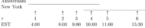
In our sample, Dutch shares traded from the Amsterdam open, 3:30 Eastern Standard Time (EST), to the New York close, 16:00 EST, with a one-hour trade overlap, as depicted in Figure 1. To study around-the-clock price discovery, the re-searcher can choose the intraday time points arbitrarily. The only concern is that the time between these points is long enough for the transitory (microstructure) effects to die out. If this is not the case, the independence of the “noise” terms
εk,t,τ across time points might be violated. We choose to select
Figure 1. Time Line. This figure illustrates the time line for trad-ing in Amsterdam and New York ustrad-ing Eastern Standard Time. The economically interesting time points modeled in this article are indi-cated with arrows. Most are self-explanatory, except for the 8:00 time point, which was introduced to pick up the potential effect of U.S. macro-announcements and premarket open press releases of rival U.S. firms.
six economically relevant time points inspired by the variance patterns reported in earlier studies (Werner and Kleidon 1996; Hupperets and Menkveld 2002). The first time point is 4:00, which is half an hour after the Amsterdam open. We choose not to take the actual open, because trading might not start directly, creating a missing observation. Subsequent time points in the Amsterdam trading period are 8:00, 9:00, and 10:00. These are, purposefully, located around the economically interesting event times 8:30 and 9:30, because at these times U.S. macroan-nouncements are published and the NYSE opens, respectively. In the U.S. trading period, we further select 11:00 to incorporate the Amsterdam close and 15:30 to study price discovery during the remainder of the trading day. We choose to stay half an hour ahead of the close to minimize disturbances due to last-minute trading. The time between each of the points is at least one hour for which we expect the transitory effects to die out. For the 30 Dow stocks, Hansen and Lunde (2006, p. 127) found that “the noise may be ignored when intraday returns are sampled at rel-atively low frequencies, such as 20-minute sampling.”
The Amsterdam and the New York stock exchanges are both continuous, consolidated auction markets in the terminology proposed by Madhavan (2000). Both exchanges release trade and quote information in real time. The main difference is that the NYSE is a hybrid market, because orders can arrive at the floor through both brokers and the electronic Superdot system. The Amsterdam Stock Exchange is a pure electronic market in which orders are routed to a consolidated limit order book and are executed according to price–time priority. In our sam-ple period, a market maker (“hoekman”) was assigned to each book with the obligation to “smooth price discovery” by insert-ing limit orders at times of illiquidity. For the blue-chip stocks we study, however, they rarely intervened. And, for our sam-ple period, tick sizes were comparable across both exchanges: U.S.$ 1/16 at the NYSE and NLG .1 (≈U.S.$ .05) at the Ams-terdam Stock Exchange.
The dataset used in this study consists of trade and quote data from Euronext–Amsterdam and the NYSE for July 1, 1997 through June 30, 1998. Seven Dutch blue-chip stocks cross-listed in New York have been selected for the current study: Ae-gon (AEG), Ahold (AHO), KLM, KPN, Philips (PHG), Royal Dutch (RD), and Unilever (UN). These firms are multination-als in different industry groups and represent more than 50% of the local index in terms of market capitalization. We use Dutch guilder–U.S. dollar (NLG–USD) tick data from Olsen & As-sociates to convert all prices to USD, which is the benchmark currency. In the robustness section, we show our results are ro-bust to prices in NLG instead of USD.
Table 1. Summary Statistics for Trading in Amsterdam and New York
Stock exchange
Share
Variable AEG AHO KLM KPN PHG RD UN
Panel A: Trading statistics full day (15-minute averages)
Trade price AMS 922 1,360 1,284 1,005 1,412 730 581
Volatility (bp2) NY 336 1,214 753 376 808 859 493
Midquote AMS 544 1,076 929 642 1,118 600 438
Volatility (bp2) NY 274 799 686 390 743 914 533
Quoted AMS 23 40 37 32 25 20 18
Spread (bp) NY 51 106 66 90 38 44 19
Effective AMS 18 26 28 25 18 15 14
Spread (bp) NY 19 49 32 35 15 15 13
Volume AMS 34 89 20 53 77 139 57
(1,000 shares) NY 3 1 6 1 24 72 20
Panel B: Trading statistics overlapping hour (15-minute averages)
Trade price AMS 1,437 2,116 2,321 1,779 2,096 1,017 966
Volatility (bp2) NY 933 2,007 1,840 733 1,508 1,291 619
Midquote AMS 1,038 1,708 1,949 1,325 1,783 897 827
Volatility (bp2) NY 888 1,466 1,679 815 1,553 1,284 710
Quoted AMS 23 41 36 31 25 21 20
Spread (bp) NY 61 120 83 90 44 47 20
Effective AMS 20 28 32 28 20 17 16
Spread (bp) NY 51 82 58 83 33 17 21
Volume AMS 53 124 33 81 123 232 95
(1,000 shares) NY 5 3 11 2 38 120 34
NOTE: This table contains summary statistics for trading in Amsterdam and New York from July 1, 1997 through June 30, 1998. Panel A contains averages for the full trading day; panel B for the overlapping hour. All variables are 15-minute averages.Trade Price Volatilityis calculated as the variance of the 15-minute squared returns based on transaction prices and measured in basis points.Midquote Volatilityis calculated the same way, but based on midquotes.Quoted Spreadis calculated as the time-weighted average of all prevailing quoted spreads in a 15-minute interval. Effective Spreadis calculated as the time-weighted average of twice the difference between the transaction price and the prevailing midquote. Both spreads are measured in basis points.Volume is the 15-minute average number of shares traded.
Summary statistics for trading in the seven Dutch stocks are shown in Table 1. They are very diverse as is apparent from trade variable averages such as volatility, volume, and spread (definitions are given in the table footnote). A closer look re-veals that they are similar in two important ways. First, for none of the stocks has New York been able to generate more volume than Amsterdam. Second, quoted spreads are larger in New York, up to almost 300%. This is most likely due to the different market structure in New York, where many or-ders receive price improvement from the floor. The effective spread, in this case, is a more appropriate measure, because it is based on actual trades. Changing to this measure, we find that differences shrink and for some stocks New York spreads are lower. Although finding the most competitive exchange is beyond the scope of this article, effective spread results show that exchanges are very competitive, which is a promising re-sult in view of the price discovery questions addressed in this study. Comparing Amsterdam to New York based on statistics for the overlapping hour yields a similar picture. The main dif-ference is that average values for all variables are higher during the overlap.
4. EMPIRICAL RESULTS
4.1 Variance Ratio Estimates
As a preliminary analysis, we follow the standard variance ratio approach and calculate the variance pattern, based on pooled intraday and overnight squared midquote returns. The intraday returns are calculated based on the six identified time
pointsτi, where we arbitrarily choose the average midquote as a
proxy for the price during the overlap. In addition to the pooled estimates, we also estimate variance patterns stock by stock to study heterogeneity. We use a Newey–West approach to cal-culate standard errors to account for commonality in (squared) returns (and, thus, deal with the Ronen 1997 critique) and po-tential nonzero autocovariances up to a one-week lead and lag period.
For all estimates reported in this article outliers were re-moved for different reasons. First, in 1998 the change to day-light savings time in the Netherlands happened one week be-fore it occurred in the United States. As a result, there was no trading overlap from March 30 to April 3, 1998. This period was removed from the sample because it was not representa-tive. The week of nonoverlap could be used to test whether the increased variance patterns are due to both markets being open simultaneously or to more information being produced exoge-nously during those times of day. Exploratory results reveal the former to be the case, but the period of one week is too small for any statistical significance. Second, at the end of the trading day on October 27, New York prices collapsed by 7%. They fully recovered at the New York open the next day. This overnight period was removed from the sample because it was a clear temporary distortion. Third, on a Unilever quarterly announce-ment on May 1, 1998, the share price jumped by roughly 8% on the Amsterdam open. This jump was removed because it clearly was a one-time event and not representative for regular around-the-clock price discovery on an “average day.”
Table 2 reports the variance estimates, which are scaled by the number of hours between time points to create hourly equiv-alents. This facilitates easy comparison across time intervals.
Table 2. Hourly Variance for Intraday and Overnight Returns
Time intervals
Event Start NY NY AMS NY
Over-AMS preopen open close only night
Start (EST) 4:00 8:00 9:00 10:00 11:00 15:30
End 8:00 9:00 10:00 11:00 15:30 4:00
Panel A: Pooled variance estimates Panel C: Pairwise variance ratio tests for pooled estimates
(Wald,χ2(1))
NOTE: This table contains estimates of the midquote return varianceσ2
τfor different intraday
time intervals based on July 1, 1997 through June 30, 1998. All stocks are included. Midquote returns are first demeaned by subtracting the time-proportional average mean over the entire sample and then scaled to correct for interstock volatility differences. Standard errors are based on a Newey–West procedure to account for nonzero autocorrelation. We use the same pro-cedure to also account for commonality across returns. Panel A presents the pooled variance estimates. Panel B presents these estimates on a stock-by-stock basis. Panel C presents pair-wise “variance ratio” tests for the pooled estimates of panel A. We test equality based on a Wald test and the Newey–West covariance matrix that accounts for intraday correlation across returns and autocorrelation up to a one-week lead and lag period.
∗Significant at the 95% confidence level.
Panel A contains the pooled estimate and shows that for the three intervals in the Amsterdam trading period, the average variance is 3.6×10⁻⁵, which corresponds to a standard devi-ation of 60 basis points per hour or an annualized volatility of 47%. Variance for the hour containing the Amsterdam close is a significant 48% higher. In the terminology of the existing lit-erature, we find that price discovery—the information flow per unit of time—in this hour is a factor of 1.5 higher (see, e.g., French and Roll 1986; Jones et al. 1994; Ronen 1997; George and Hwang 2001). Additionally, the Amsterdam nonoverlap is a significant of factor 2.4 more informative than the NYSE nonoverlap, which, in turn, is a significant factor of 1.3 more informative than the overnight hours. Panel B reports the stock-specific patterns and illustrates the heterogeneity of the sample. For six out of seven stocks, we find that the Amsterdam close continues to be the most informative period. The result that the New York only is more informative than the overnight, how-ever, only holds for four stocks. Straightforward pooling, as is often done in the literature, does not seem to be appropriate for our sample. Also note that Royal Dutch (RD) as opposed to the other stocks has a variance for the New York only period that is roughly equal to that of the Amsterdam only period. This is due to the proportionally higher trading volume of RD on the
Table 3. Intraday Return Autocorrelations
Time interval Event Lag 1 Lag 2
4:00–8:00 AMS only −.077
8:00–9:00 NY preopen .056 −.020 9:00–10:00 NY open −.125∗ −.005 10:00–11:00 AMS close .251∗ −.170∗ 11:00–15:30 NY only −.050 .039 15:30–4:00(+1) Overnight −.165∗ −.022
NOTE: This table presents the raw return autocorrelations up to the second lag of intraday and overnight midquote returns. The midquote in the overlapping interval was arbitrarily fixed at the average of the Amsterdam and New York midquotes. The autocorrelations are calculated for the full sample period, from July 1, 1997, through June 30, 1998, and averaged across all stocks. We explicitly account for commonality in returns when determining confidence intervals.
∗Significant at the 95% confidence level.
NYSE. In the advocated state space approach, we control for heterogeneity across stocks through a stock-specific variance parameter (ci), differential factor loadings on a common factor
(βi), and, in a robustness check, stock-specific variance of the
microstructure effects. In the extreme case, we could abstain from pooling altogether and estimate the model on a stock-by-stock basis. In that case, however, it would no longer be possi-ble to distinguish the market reaction to common versus stock-specific information. We, therefore, do not pursue this line of research further.
To further motivate the state space model advocated in this article, Table 3 reports the autocorrelations for intraday returns. If measurement errors exist and if they are economically signif-icant, we should find negative first-order autocorrelation. Most of these autocorrelations are indeed negative and two of them are significant. We find a significantly positive autocorrelation for the period containing the Amsterdam close. Apparently, markets underreact to information in the New York open, caus-ing persistence in returns for the subsequent Amsterdam close period. Higher order autocorrelations are insignificant, except for the Amsterdam close period.
4.2 Estimation Results
We proceed by re-estimating the intraday variance pattern us-ing the state space model advocated in this article. We test for significance of parameters at a 95% level and omit the insignif-icant ones. Furthermore, we scale our (innovation) variance es-timates by the number of hours between time points to create hourly equivalents, which facilitates easy comparison across time intervals. The results are shown in Tables 4 and 5.
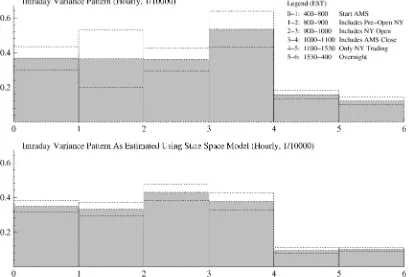
Panel A of Table 4 presents the estimate of the variance pat-tern of the efficient price, which is plotted in Figure 2 along with the variance pattern based on the direct variance ratio ap-proach reported in Table 2. The state space model estimates dif-fer in two important ways. First, most information is attributed to the New York open, instead of the Amsterdam close period. The reason is market underreaction to both common-factor and firm-specific information (35% and 34%, respectively) in the New York open period. In other words, the efficient price in-novation in the New York open period is not yet fully revealed in midquotes halfway through the overlapping period. We con-jecture that this is due to informed investors who trade strate-gically and split their order over time to maximize profit. They might have a preference for trading in the overlapping period
Table 4. Estimation Results for Efficient Price and Observation Models
Panel A: Variance efficient price innovation (×10,000, hourly) Time intervals
Event Start NY NY AMS NY
Over-AMS preopen open close only night
Start (EST) 4:00 8:00 9:00 10:00 11:00 15:30
End 8:00 9:00 10:00 11:00 15:30 4:00
σE2,τ .35 .33 .43 .38 .09 .10 (.02) (.02) (.02) (.03) (.01) (.01) σξ,τ2 .13 .18 .16 .15 .05 .05
(.01) (.02) (.02) (.02) (.01) (.01)
θξ,τ −.35 −.16
(.04) (.04) ση2,τ .22 .15 .27 .23 .05 .05
(.01) (.01) (.01) (.02) (.01) (.00) θη,τ −.34 −.30 .87
(.02) (.08) (.13)
Panel B: Variance measurement error (×10,000) Time points (EST)
Start (EST) 4:00 8:00 9:00 10:00 11:00 15:30
σε2,A,τ .00 .00 .00 .07 (.00) (.00) (.00) (.01)
σε2,NY,τ .11 .07 .14 (.01) (.02) (.00)
NOTE: This table contains maximum likelihood estimates of the state space model (1) and (7) based on intraday midquotes for July 1, 1997 through June 30, 1998. The observation vector
pk,t,τcontains the midquotes for all stocks traded in marketkat daytand time pointτ. Panel A contains estimates of the efficient price innovation varianceσ2
E,τ, the common price variance σ2
ξ,τ, the response to a common innovationθξ,τ, the firm-specific price varianceση2,τ, and the
response to a firm-specific innovationθη,τ. Note thatσE,τ2 =σξ,τ2 +ση2,τ. Panel B contains
esti-mates of measurement error variance in both markets,σ2
ε,k,τwithk∈ {A, NY}. Standard errors
are in parentheses.
as they can hide their order flow by trading across two mar-kets (see Kyle 1985 for informed trader behavior in a single market and Chowdhry and Nanda 1991 and Menkveld 2005 for a multiple-markets setting). This behavior could also explain the market underreaction (30%) to firm-specific information in the Amsterdam close period. Second, trading in New York af-ter the Amsaf-terdam close isnotsignificantly more informative than the overnight nontrading hours. The main reasons are that the New York midquotes contain significant transitory effects and that the New York market appears to overreact significantly (87%) to firm-specific information. The overreaction is most likely due to increased market-making activity by the NYSE specialist after the home market, as a secondary pool of liquid-ity, disappears. Moulton and Wei (2005) studied NYSE trading of European stocks and documented a significant increase (6%) in specialist participation rates after the home markets close. We also find that the market underreacts to common-factor in-formation, but this effect is much smaller (16%) and, as we will show later, is not robust.
We conduct formal tests of equality of the over-/underreac-tion coefficients for firm-specific and common-factor informa-tion. We cannot reject the hypothesis of an equal coefficient for the New York open period [H0:θξ,τ =θη,τ in model (7) forτ
corresponding to the New York open period]. Theχ2(1)Wald test for this hypothesis has a value of .025. For the New York only period, however, this test has a value of 95.6, which clearly rejects the null of equal coefficients. It is, therefore, important that the model allow for a different market reaction to common-factor relative to firm-specific information.
Figure 2. Raw Return Variance versus State Space Innovation Variance. The top figure illustrates the estimate of the intraday variance pattern based on raw returns of all stocks, taking into account interstock volatility differences. It is presented on an hourly basis to enhance comparability. The bottom figure represents the variance pattern based on the returns of the unobserved efficient price as estimated by the state space model. The bars represent point estimates; the dotted lines 95% confidence intervals.
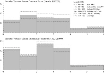
Figure 3. Variance Decomposition Into Common and Idiosyncratic Components. The state space model specification allows for decomposition of the efficient price returns into two components: a common component due to a common (market-wide or macro) factor driving the returns across all stocks and an idiosyncratic component due to firm-specific returns. Hence, the variance can be decomposed by time of day. The efficient price variance pattern, as depicted in Figure 2, is, therefore, the sum of two components: The top figure represents the common-factor component; the bottom figure the stock-specific or idiosyncratic component. The bars represent point estimates; the dotted lines 95% confidence intervals.
To characterize around-the-clock price discovery in more de-tail, we further decompose information into firm-specific and common-factor information by the time of day. Figure 3 illus-trates this decomposition and leads to three important observa-tions. First, the significantly larger innovations in the efficient price during the overlap are due to increased firm-specific rather than common-factor information. Apparently, a disproportion-ate amount of firm-specific information is produced through trading in this period. This is consistent with our earlier conjec-ture on increased informed trading in the overlap. An alternative explanation is that the opening prices of U.S. peers are infor-mative on the state of the industry. Second, the New York pre-opening period is characterized by common-factor rather than firm-specific information. Although this period is not signifi-cantly more informative than the preceding Amsterdam trad-ing hours, its common-factor component is significantly higher and its firm-specific component is significantly lower. Third, we find for neither the firm-specific nor the common-factor compo-nent that the New York only period is more informative than the overnight period. This finding is consistent with Craig, Dravid, and Richardson (1995) who found that only a small portion of overnight volatility in the Nikkei index occurred during U.S. trading hours.
In panel B of Table 4, we report the variance of the transi-tory effects. In the optimization, they converge to 0 for all time points in Amsterdam outside the overlap. We cannot reject the null of no such effects for these midquotes. For the New York midquotes outside the overlap, however, we do reject the null
of no transitory effects. During the overlap both the Amster-dam and the New York midquotes are affected by significant transient components. The New York quotes, however, are sig-nificantly noisier than the Amsterdam midquotes. The estimates imply a 33-basis-point standard deviation for New York errors, which is 26% higher than the standard deviation of Amsterdam errors. This, together with the nonoverlap results, shows that home market trading produces more efficient price discovery. The errors are economically significant because they are of the same magnitude as hourly efficient price innovations.
Table 5 reports the stock-specific parameter estimates of the vector of loadings β and the scaled variance matrixC in the price model (1). For five out of seven stocks, the estimate ofβ
Table 5. Estimation Results for Decomposition Parameters
Share
Parameter AEG AHO KLM KPN PHG RD UN
βi .98 1.23 .87 .87 1.11 1.00 .88
(.03) (.03) (.04) (.03) (.04) (.03) (.04)
ci .55 1.21 1.54 .67 1.83 .75 .46
(.03) (.06) (.06) (.03) (.07) (.04) (.03) βi2/ci 1.75 1.25 .49 1.12 .68 1.34 1.68
(.16) (.10) (.05) (.10) (.06) (.11) (.15)
NOTE: This table contains maximum likelihood estimates of the state space model (1) and (7) based on intraday midquotes for the period from July 1, 1997 through June 30, 1998. The model is for observation vectorpk,t,τthat contains the midquotes for all stocks traded in market kat daytand timepointτ. Estimates are presented for the common factor loading vectorβand diagonal variance matrix of firm-specific innovations. For ease of interpretation, the common factor variation relative to firm-specific variation is measured byβ2
i/ci for stocki=1, . . . ,n.
Standard errors are in parentheses.
differs significantly from 1. Comparing these with “standard” betas based on simple linear regressions of daily returns on the index, we find a correlation of almost .80. The correlation is not perfect becauseβmeasures different exposures—high- ver-sus low-frequency exposures to market-wide “shocks” or macro factors. Cross-sectional variation is even higher for interstock variance differences measured byCbecause this parameter dif-fers significantly from 1 for every stock. Given this heterogene-ity inβ and in the variance matrix C, the general pattern re-ported in Figure 3 should be interpreted carefully. Whereas it is informative on the intraday pattern of both components, it is not informative on how important both components are for a specific stock. To find the decomposition into these compo-nents for stock i, we multiply the ratio of reported common and idiosyncratic variance (for the “average” stock) with the factorβi2/ci. These factors are reported in Table 5 and, not
un-expectedly, vary significantly across stocks. Interestingly, the common-factor component is highest for Aegon, Royal Dutch, and Unilever. This is probably due to these stocks’ high ex-posure to the U.S. market in our sample period, because Aegon just took over the U.S. company Transamerica and Royal Dutch and Unilever were members of the S&P500.
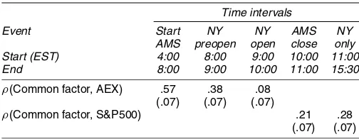
Finally, the state space approach provides us with an estimate of the common factor conditional on the observations. We can compare this with local market indices—the S&P500 and the AEX—for each time of day. In Table 6 we report the corre-lation between this common-factor estimate and index returns. The correlation is highest, .57, and significant for the start of the trading day in Amsterdam. The correlation is, perhaps, surpris-ingly low, because our stocks represent more than 50% of the index in terms of market capitalization. An important reason is that the weight each of these stocks has in the index is capped. The correlation drops significantly to .38 in the New York pre-open, indicating that the cross-listed stocks,collectively, start price discovery diverging from the remainder of the Dutch mar-ket. This effect is particularly strong for the hour containing the NYSE open, because correlation with the AEX now drops to an insignificant .08. For the remainder of the trading day, the com-mon factor significantly correlates with the S&P500 with cor-relation coefficients of .21 and .28. These levels are lower than the Amsterdam nonoverlap, because these stocks, obviously, do not make up a significant part of the S&P500. Interestingly, the correlation with the local market is higher outside the over-lap than during the overover-lap. Halling, Pagano, Randl, and Zech-ner (2005) discussed the geographic distribution of informed
Table 6. Correlation Common Factor and Market Index
Time intervals
Event Start NY NY AMS NY
AMS preopen open close only
Start (EST) 4:00 8:00 9:00 10:00 11:00
End 8:00 9:00 10:00 11:00 15:30
ρ(Common factor, AEX) .57 .38 .08 (.07) (.07) (.07)
ρ(Common factor, S&P500) .21 .28 (.07) (.07)
NOTE: This table contains the correlations between the common-factor estimate conditional on all observed data—often referred to as the “smoothed estimate” (see, e.g., Durbin and Koop-man 2001, p. 16)—and intraday returns on the AEX index and the S&P500 indices for different intraday time intervals. Standard errors are in parentheses.
trading and recognized that foreigners might be at a disadvan-tage for information that is produced locally, but argued that there might be instances where a considerable portion of value-relevant information is produced abroad. They argued that this can occur when the company exports or produces abroad a large fraction of its output or when its major suppliers or competi-tors are located abroad. These conditions hold for most of the (Anglo-)Dutch multinationals. Baruch, Karolyi, and Lemmon (2003) formalized this argument in their model by making in-novations in the cross-listed security correlate with inin-novations in the local and foreign markets. This could explain our intra-day correlation pattern, because shares correlate higher with a market index when no additional information arrives from the other market, that is, outside the overlap.
4.3 Discussion of Results
In this section we focus on the robustness of our main results and discuss the model assumption that measurement error is independent of the efficient price innovation, which is at odds with some of the microstructure literature. Although all results are discussed in this section, we only report the most important results in a summary table to conserve space. The results that are not reported here are available upon request.
Because our primary interest in the article is around-the-clock price discovery, we test robustness of the estimated intra-day variance pattern into two ways. First, we split the sample in two subperiods and estimate the model for each period. Second, we estimate the model converting all quotes to Dutch guilders instead of U.S. dollars. The results, reported in panels B and C of Table 7, show that the main results are largely unaffected, that is, the around-the-clock information pattern, the market under- and overreaction parameters, and the significantly larger transitory effects in the overlap NYSE prices. The only differ-ence is that the common-factor underreaction during New York only trading vanishes in the second subperiod. Interestingly, we find that the volatility of innovations is larger for all subperiods when using prices in Dutch guilders, which indicates that the U.S. dollar is, indeed, the benchmark currency for these multi-nationals.
The assumed independence of the efficient price innova-tion and the transitory effect seems at odds with common mi-crostructure models. In a standard structural model, the transac-tion price at timetequals the sum of an efficient price and a lin-ear expression in signed volume of the previous two trades (see, e.g., George and Hwang 2001, p. 981). Because the innovation in the efficient price is a linear function of the same signed vol-umes (plus additional terms), the independence assumption for
εk,t,τ andηt,τ in our state space model could be violated.
Ide-ally, we would relax the assumption to test the robustness of our results, but this is, econometrically, not possible because the model would become unidentified (see also Hasbrouck 1993). Instead, we argue that it is unlikely that the issue impacts our main results for three reasons. First, we model midquotes in-stead of transaction prices, which eliminates one of the signed volume terms in the “transaction price” equation. Second, the remaining signed volume term relates to the cost for a single market maker to carry inventory through time. This is not an is-sue for the Amsterdam market because it is fully electronic and
Table 7. Robustness Checks
σE2,τ θξ,τ θη,τ σε2,A,τ σε2,NY,τ
Start NY NY AMS NY Over- NY NY NY AMS NY
AMS preopen open close only night open only open close only
4:00 8:00 9:00 10:00 11:00 15:30 9:00 11:00 9:00 10:00 11:00
8:00 9:00 10:00 11:00 15:30 4:00 10:00 12:00 10:00 11:00 15:30 10:00 10:00
Panel A: Basic model .35 .33 .43 .38 .09 .10 −.35 −.16 −.34 −.30 .87 .07 .11 (.02) (.07) (.02) (.01) (.01) (.00) (.04) (.04) (.02) (.08) (.13) (.01) (.01)
Panel B: Subperiods
First .41 .48 .51 .43 .11 .09 −.40 −.25 −.39 −.36 1.13 .08 .12 (.03) (.04) (.04) (.04) (.01) (.01) (.05) (.04) (.03) (.10) (.24) (.00) (.01) Second .28 .18 .39 .31 .08 .10 −.23 .00 −.31 −.17 .66 .06 .09
(.02) (.01) (.03) (.03) (.01) (.01) (.09) (.00) (.03) (.15) (.14) (.00) (.01)
Panel C: NLG instead of USD
.42 .35 .54 .44 .10 .11 −.35 −.15 −.34 −.25 .83 .08 .10 (.02) (.02) (.03) (.03) (.01) (.01) (.04) (.04) (.02) (.08) (.12) (.00) (.01)
Panel D:ρ=.175
.35 .33 .41 .32 .08 .10 −.32 −.16 −.31 −.31 .63 .07 .11 (.02) (.02) (.02) (.02) (.01) (.01) (.04) (.04) (.02) (.07) (.09) (.00) (.01)
NOTE: This table contains estimates of the efficient price innovation variance and other parameters for various models. They represent robustness checks of the main results of Table 4. Panel A repeats the estimates of Table 4. Panel B splits the sample into two subperiods: (1) July 1, 1997–December 31, 1997 and (2) January 1, 1998–June 30, 1998. Panel C uses prices in NLG instead of USD. Panel D sets the correlationρ(ηt,τ−1,εk,t,τ) between the efficient price innovation and the subsequent measurement error equal to .175, inspired by microstructure theory and empirical
work by George and Hwang (2001). Standard errors are in parentheses.
highly liquid, so that virtually all trades are executed without the intervention of the designated market maker (“hoekman”). In New York, however, the market maker (“specialist”) is an active intermediary. Madhavan and Sofianos (1998) reported a mean participation for U.S. stocks of 25% for 1993. Moulton and Wei (2005) studied 2003 NYSE trading in European stocks and documented a mean specialist participation rate of 34% in the overlap and 40% in the nonoverlap. The overreaction we find for the firm-specific information in the nonoverlap is con-sistent with active inventory control. Interestingly, we do not find such overreaction to the common-factor component, which is not surprising because common factors are easier to hedge. New York results, therefore, could be affected.
Third, panel D in Table 7 shows that the main results are not affected by presetting the correlation to .175, which is our best guess based on George and Hwang (2001). In their ta-bles 5 and 6, they reported that 9% of the transitory compo-nent (“measurement error”) variance and 34% of the permacompo-nent component (“efficient price innovation”) are due to signed vol-ume. Because all correlation between the two components is driven by the stochastic signed volume factor, sayα, we iden-tify the correlation between both components as
ρ(ε, η)=cov(ε, η) σεση =
σα2
σα √
.09 σα √
.34
≈.175
where we assume positive correlation between the two compo-nents, consistent with compensation for inventory holding by (implicit) market makers.
5. CONCLUSION
This article studies around-the-clock price discovery for cross-listed stocks in markets that do not fully overlap. We pro-pose a state space model for multiple stocks with an efficient price as the unobserved state and midquotes as observations. Compared to other approaches, the model’s relative strength is
in its ability to deal naturally with (1) simultaneous quotes in an overlapping period, (2) missing observations in the nonover-lap, (3) transient price changes due to short-term microstructure effects, and (4) contemporaneous correlation in returns due to common market-wide factors. The model is rich in that it al-lows us to estimate the efficient price (and its innovations) con-ditional onalldata. An example is our estimate of the common-factor innovation by time of day, which we correlate with local market returns to identify to what extent the common factor mirrors the Dutch or U.S. market return.
We exploit a rich dataset on Dutch stocks cross-listed on the NYSE with tick data on trades, quotes, exchange rates, and both local market indices. We find that the overlapping period is the most important period in 24-hour price discovery, followed by the Amsterdam only (home market) period. Least important are the New York only and the overnight period, which, perhaps surprisingly, are equally uninformative. Further evidence of the NYSE’s minor role in price discovery are the significant tempo-rary effects throughout the trading day. Amsterdam midquotes, however, are not affected by these effects outside the overlap and significantly less during the overlap.
The around-the-clock price discovery process can be further analyzed by decomposing the information by time of day into a firm-specific component and a common-factor component. We find that it is firm-specific information that causes the overlap to be relatively more informative. The common-factor estimate correlates highly with the Dutch market index in the early Ams-terdam hours, but this correlation decreases substantially in the course of the day, as we get closer to the start of trading in New York. The correlation is low and insignificant around the New York open, indicating that the cross-listed stocks exhibit com-mon price discovery independent of the rest of the home mar-ket. During New York trading hours, the common factor signif-icantly correlates with the S&P500. Again, this correlation is lower during the overlap than outside the overlap. These find-ings are consistent with Halling et al. (2005) and Baruch et al.