EVALUATION OF EROSION BASED ON GIS AND REMOTE
SENSING FOR SUPPORTING INTEGRATED WATER RESOURCES
CONSERVATION MANAGEMENT
(Case Study: Manjunto Watershed, Bengkulu Province-Indonesia)”
Gusta Gunawan1, Dwita Sutjiningsih1 , Herr Soeryantono1, Sulistioweni.W1 1Department of Civil Engineering, Faculty of Engineering
University of Indonesia, Depok, West Java 16424 INDONESIA
E-mail : [email protected], [email protected], [email protected]
Abstracts :
Soil erosion is a crucial environmental problem in the Manjuto watershed. It has economic implications and environmental consequences. Assessment of soil erosion risk is useful to design soil conservation strategies for integrated watershed management. Information obtain from RS and GIS framework can help decision makers prepare spatial maps accurately in less time and cost. The aims of this research are to assess the average annual rate of soil erosion in Manjunto Watershed on the each soil mapping unit. The average annual rate of soil erosion rate was estimated using Remote Sensing data. The basis data used NDVI and Slope. The value of NDVI obtained from satellite imagery processing and Slope value obtained from the DEM processing. The results showed that the eroded catchment area has increased significantly. The average annual rate of soil erosion in the watershed Manjunto in 2000 amounted to 3.00 tons ha-1 year-1. It was an increase to 27.03 ton ha-1 year-1 in 2009. The levels of erosion hazard are very heavy category in soil mapping unit number 41, 42 and 47. It should be a first priority in the soil and water conservation activities.
Keywords:Soil erosion, Remote Sensing, GIS, DEM, NDVI.
I. INTRODUCTION
Watershed management system which is unintegrated, has led to high soil erosion, thus increasing the number of critical watershed and critical land area in Indonesia significantly. The number of critical watershed is currently more than 62 critical watersheds and critical land area of about 30.2 million ha, of which 23.3 million ha of land classified as highly critical category (Statistics Department of Forestry, 2010). The factors that caused of high soil erosion are the use of land that is not in accordance with its carrying capacity, techniques of farming that do not correspond to the rules of conservation, high rainfall, topography, and slope (Asdak, 2009).
and to determine the effective action in priority setting and location of conservation programs (Morgan, 2005).
Rapid development occurring in the technology of Remote Sensing (RS) and Geographic Information Systems (GIS) provide a new approach to meet various demands related to the modeling of resources (Mermut and Eswaran, 2001 Salehi et al., 2003) including soil and water conservation (Hazarika et al, 2009). Green (1992) stated that the integration of RS in a GIS database can reduce costs, reduce time and improve the detailed soil survey information. Therefore, the use of the technology of Remote Sensing and Geographic Information Systems in watershed management will vastly assist managers in making decisions. Satellite data can be used for mapping, monitoring and estimation of soil erosion (Hazarika & Honda, 2001).
Although soil erosion mapping using GIS and RS conducted in many countries, such as those conducted by Spanner et al (1982) which combines GIS with USLE for soil erosion and loss assessment. Hazarika and Honda (1999) mapped the threat of erosion in Thailand to evaluate the conservation activities in Mae Ao watershed, northern Thailand. Milevsky (2008) introduced a GIS method to estimate soil erosion in the watershed based digital elevation model (DEM) and satellite imagery analysis. Ande et al (2009) approach to estimate the erosion Morgan and Finney Model (MMF) in Southwest Nigeria. Kevi and Yoshino (2010) using RUSLE, remote sensing and GIS to estimate the hazard of erosion on agricultural productivity in watershed Tunisia. However, erosion mapping studies have not been carried out extensively in Indonesia (Arsyad, 2010). Map of soil erosion that published is the mapping performed by Dames (1955) by using traditional methods in the watershed of Central Java, which covers 1.6 million hectares. The use of GIS to evaluate land degradation first performed by Lanya (1996), estimated rates of soil erosion that occurs done by identifying morphological changes in the soil in-situ.
The aim of this research is to evaluate the potential of soil erosion on a watershed scale using E30 models in each Soil mapping unit. The result of this study expected to be used as guidelines for the determination of strategy and site selection that will be the main priority on soil and water conservation activities. The selection model based on the condition of land cover in the study area.
II. MATERIALS AND METHODS
2.1. Location and Description of Study Area
2.4. Estimate of Soil Erosion with E30 Model
To estimate the hazard of soil erosion that occur in each soil mapping unit used the following equation (Hazarika and Honda, 2001):
(
)
0.9 30 30 S SE
E= (1)
Where E = rate of annual soil erosion in the Manjunto watershed (ton ha-1year-1), S = gradient of the point under consideration (%), S30 = Tan (300), and E30 = the rate of soil erosion that occurs on a slope of 300, obtained using equation 2 (Hazarika and Honda, 2001).
(
)
⎥30 exp NDVI NDVI LogE
NDVI NDVI
LogE LogE
E (2)
The maximum erosion values and the minimum obtained from the data of the Public Works Department of Bengkulu Province; Emax is 242 tons ha-1 year-1 and Emin is 0.1 tons ha-1 year-1. NDVI can be calculated from the satellite image of the ratio calculations constructed from two spectral channels, namely spectral infra red (IR) and near infra red (NIR). The general equation of NDVI as follows (Honda, 2001; Panuju, et al, 2009) :
NDVI=(IR-NIR)/(IR+NIR) (3)
If the channel, that recording infrared wave is Band 4 (B4) and near infrared wave are Band 3 (B3), so the equation 3 can be changed as equation 4. To avoid negative values and for easy handling of digital data, NDVI values re-scale, so the NDVI equation is as follows:
100
3. RESULTS AND DISCUSSION
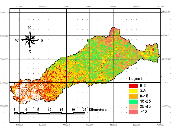
3.1. The slope Map
Slope map of DEM processed with the help of Arc Gis 9.3 present in Figure 2.
Figure 2. The slope map of Manjunto Watershed
Data processed by GIS contains information on slope and the number of pixels or extensive information. Information about slope of it presented in Table 1.
Table 1. The slope of the watershed Manjunto
No. Slope Class
(%)
Area Persentage
(Ha) (%)
1 0 - 8 20,923.88 26.292 2 8 - 15 31,949.35 40.147 3 15 - 25 15,155.85 19.045 4 25 - 45 5,667.83 7.122
5 > 45 5,883.77 7.393 79.580,678 100,000
The mayor of study site has the slope above 8%. The Slope factor will influence the speed and volume of surface runoff. Small slope will provide more opportunities the water rain to infiltration so that runoff volume will reduce. In the other side, a low percentage of slope will reduce runoff velocity so that its ability to erode and transport the soil to be small.
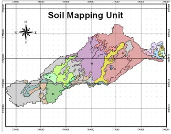
3.2. Soil Mapping Unit (SMU)
Figure 3. Soil Map Unit of Manjunto Watershed
Most of the study area has the slope above 8%. Slope affects the speed and volume of surface runoff. Small slope will provide more opportunities to the rain water to infiltration so that runoff volume will be low. Small slope will reduce runoff velocity so that its ability to erode and transport the soil also will be small.
3.3. Land Cover
Based on the identification of land cover in 2000 and 2009, it is showing that the conversion of land use and the reduction of forest from deforestation. Changes in land use can be seen at Figure 4 and 5.
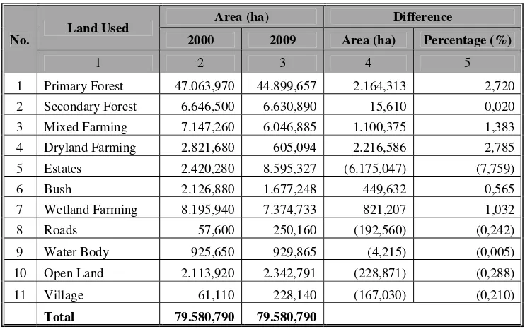
Land cover changed on every class of land use shown by Figure 4 and 5. The total area of forest significantly reduced, while the plantation or estates area increased significantly. Changes in land use influenced by the local livelihoods of the majority are as a farmer. The detail of Land use conditions shown in Table 2.
Table 2. Land Cover Conditions of Manjunto Watershed in 2000 and 2009
No. Land Used
Area (ha) Difference
2000 2009 Area (ha) Percentage (%)
1 2 3 4 5
1 Primary Forest 47.063,970 44.899,657 2.164,313 2,720
2 Secondary Forest 6.646,500 6.630,890 15,610 0,020
3 Mixed Farming 7.147,260 6.046,885 1.100,375 1,383 4 Dryland Farming 2.821,680 605,094 2.216,586 2,785
5 Estates 2.420,280 8.595,327 (6.175,047) (7,759)
6 Bush 2.126,880 1.677,248 449,632 0,565
7 Wetland Farming 8.195,940 7.374,733 821,207 1,032
8 Roads 57,600 250,160 (192,560) (0,242)
9 Water Body 925,650 929,865 (4,215) (0,005)
10 Open Land 2.113,920 2.342,791 (228,871) (0,288)
11 Village 61,110 228,140 (167,030) (0,210)
Total 79.580,790 79.580,790
The information obtained from Table 2 that has been a change of each land cover. The percentage reduction in the area of some land cover is primary forest (2.72%), secondary forest (0.02%), mixed farms (1.383%), Dryland Farming (2.785%) and Wetland Farming (1.032%). Addition of a couple of percentage land cover is estate (3.041%), road (0.242%), open land (0.288%) and villages (0.21%). Changes in land cover strongly influenced by socio-economic conditions and local culture. The main factors affecting changes in land cover is a source of livelihood. Most of the people who live in Manjunto Watershed is farmers.
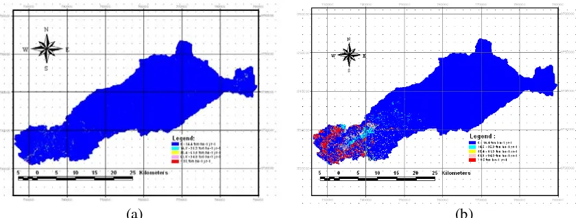
3.4. Soil Erosion Mapping
(a) (b)
Figure 6. Map of average annual erosion in the year 2000 (a) and 2009 (b)
From Figure 6 above known that the watershed area eroded increased when compared with conditions in 2000. Total amount of lost land in the watershed Manjunto 2000 at 1,399,209 tons and in 2009 amounted to 23,004,391 tons. Erosion rate of the annual average in 2000 is a 3 tons ha-1 year-1, and 2009 was 27 tons ha-1 year-1. High erosion occurs in the lower reaches of the basin's land use types, namely Dryland Farming. Factors causing the high rate of erosion is a way of farming that pays little attention to the rules of conservation and high rainfall.
To determine the level of soil erosion that occurs in each of soil mapping unit then soil mapping unit overlay with maps of soil erosion, the results as exhibited in Table 3 (attachment 1).
The planning of soil and water conservation need the information of average annual rate of soil erosion on soil mapping unit. The location of priority can be selected based on the dignity of the danger of erosion or erosion hazard index value. The location is the top priority is to have the level of danger of erosion or erosion hazard index is the highest. From Table 3 above know the number 41, 42 and 47 of soil mapping unit are a first priority for conserve, numbers 40 and 45 the soil map unit is the second priority for conserve. The selection of conservation strategies should be adapted to the socio-economic conditions and local culture.
4. CONCLUSION
The conclusion of this study are the eroded catchment area has increased significantly. The average annual rate of soil erosion in the watershed Manjunto in 2000 amounted to 3.00 tons ha-1 year-1. It was an increase to 27.03 ton ha-1 year-1 in the year 2009. Some soil mapping unit has the levels of erosion hazard are very heavy category. It should be a priority in the soil and water conservation activities. To reduce the rate of erosion is happening we need a system of sustainable agriculture and conservation management systematically.
5. REFERENCES
Ananda, J. Herath, G. and Chisholm, A. 2003. Determination of yield and Erosion Damage Functions Using Subjectivly Elicited Data: application to Smallholder Tea in Sri Lanka. The Australian Journal of Agricultural an Resources Economics, 45:2, p.275-289.
Ande O. T., Alaga Y. and Oluwatosin G. A. 2009. Soil erosion prediction using MMF model on highly dissected hilly terrain of Ekiti environs in southwestern Nigeria. International Journal of Physical Sciences Vol. 4 (2), pp. 053-057, February, 2009.
Arsyad , S. 2010. Konservasi Tanah dan Air. IPB Press. Bogor-Indonesia (in Indonesian).
Asdak C.1995. Hydrology and Watershed Management. Gadjah Mada University Press, Yogyakarta.
Dames TWg. 1955. The Soils of East Central Java; with a Soil Map 1:250,000. Balai Besar Penjelidikan Pertanian, Bogor, Indonesia.
FAO/Unesco., 1974.
Green, K .1992.Spatial imagery and GIS: integrated data for natural resource management. J. For. 90: 32-36.
Hazarika, M.K & Honda, H. 2001. Estimation of Soil Erosion Using Remote Sensing and GIS, Its Valuation & Economic Implications on Agricultural Productions. The 10th International Soil Conservation Organization Meeting at Purdue University and the USDA-ARS Soil Erosion Research Laboratory.
Honda, K. L. Samarakoon, A. Ishibashi. Y. Mabuchi. And S. Miyajima. 1996. Remote Sensing and GIS technologies for denudation estimation in Siwalik watershed of Nepal,p. B21-B26. Proc. 17th Asian Conference on Remote Sensing, Colombo, Sri lanka. 4-8 November 1996.
Kefi, M and Yoshino, K. 2010. Evaluation of The Economic Effects of Soil Erosion Risk on Agricultural Productivity Using Remote Sensing : Case of Watershed In Tunisia, International Archives of the Photogrammetry, Remote Sensing and Spatial Information Science, Volume XXXVIII, Part 8, Kyoto Japan 2010.
Kefi, M., Yoshino, K., Zayani, K., Isoda, H., 2009. Estimation of Soil Loss by using combination of Erosion Model and GIS : Case of Study Watersheds in Tunisia. Journal of Arid Land Studies, 19(1), Special issue: Proceedings of Desert Technology IX, pp. 287-290
Lal, R .1998. Soil erosion impact on agronomic productivity and environment quality: Critical Review. Plant Sci. 17: 319 – 464.
Lal., 2001. Soil Degradation by Erosion. Land Degradation and Development,12,pp. 519 – 539.
Lanya I. 1996. Evaluasi Kualitas lahan dan Produktivitas Lahan Kering Terdegradasi di Daerah Transmigrasi WPP VII Rengat Kabupaten Indragiri Hulu, Riau. [Disertasi Doktor]. Program Pasca Sarjana IPB, Bogor (in Indonesian).
Lillesand, T.M., Kiefer, R.W., 1994. Remote sensing and Image Interpretation, 3rd edition. Jhon Wiley & Sons, Inc.
Malingreau, 1986.
Mermut AR and H Eswaran. 2001. Some major developments in soil science since the mid 1960s.
Geoderma 100: 403-426.
Mongkolsawat, C., Thurangoon, P. Sriwongsa .1994. Soil erosion mapping with USLE and GIS. Proc. Asian Conf. Rem. Sens., C-1-1 to C-1-6.
Morgan, 2005
Morgan RPC, Morgan DDV, Finney HJ .1984. A predictive model for the assessment of erosion risk. J. Agric. Eng. Res. 30: 245 – 253.
Panuju DR, F Heidina, BH Trisasongko, B Tjahjono, A Kasno, AHA Syafril. 2009. Variasi nilai indeks
vegetasi MODIS pada siklus pertumbuhan padi. J.Ilmiah Geomat. 15, 9-16 (in Indonesian).
Puslitanah Bogor (1982)
Salehi MH, Eghbal MK and Khademi H. 2003. Comparison of soil variability in a detailed and a reconnaissance soil map in central Iran. Geoderma 111: 45-56.
Spanner et al (1982)
Statistics Department of Forestry, 2010
Pimentel, D., et al. 1995. Environmental and Economic Costs of Soil Erosion and Conservation Benefits. Econ61, 267,pp.1117-1123.
Renard, K.G., et al., 1997. Predicting Soil Erosion by Water: A Guide to Conservation Planning with the Revised Universal Soil Loss
Renzetti, S. 2006. Canadian agricultural water use and management. Department of Economics Working Paper Series, Brock University, Canada.
Saha SK, Kudrat M, Bhan SK .1991. Erosional soil loss prediction using digital satellitee data and USLE,. In Applications of Remote Sensing in Asia and Oceania – environmental change monitoring (Shunji Murai ed.). Asian Association of Remote Sensing pp. 369-372.
Attachement 1. Table 3. The average erosion rate of the annual soil mapping unit.
SMU Number
The Mean
Erosion Erosion
Hazard
The Mean
Soil Loss Hazard Erosion Index
The Dignity Erosion Hazard Index
(ton/ha/year) (mm/year)
(1) (2) (3) (4) (5) (6)
1 7,36 Very Low 0,74 0,28 Low
2 31,51 Low 3,15 1,19 Middle
3 7,89 Very Low 0,79 0,30 Low
6 25,64 Low 2,56 0,97 Low
9 0,13 Very Low 0,01 0,00 Low
10 0,48 Very Low 0,05 0,02 Low
11 0,36 Very Low 0,04 0,01 Low
12 0,11 Very Low 0,01 0,00 Low
13 0,59 Very Low 0,06 0,02 Low
14 1,22 Very Low 0,12 0,05 Low
15 0,17 Very Low 0,02 0,01 Low
16 0,17 Very Low 0,02 0,01 Low
19 1,17 Very Low 0,12 0,04 Low
20 1,42 Very Low 0,14 0,05 Low
21 0,15 Very Low 0,01 0,01 Low
24 1,79 Very Low 0,18 0,48 Low
25 0,03 Very Low 0,00 0,00 Low
27 1,33 Very Low 0,13 0,05 Low
28 1,47 Very Low 0,15 0,06 Low
29 1,71 Very Low 0,17 0,06 Low
33 1,82 Very Low 0,18 0,83 Low
40 48,36 Middle 4,84 1,83 Middle
41 153,33 Very Heavy 15,33 5,81 High
42 219,58 Very Heavy 21,96 8,32 High
43 1,22 Very Low 0,12 0,05 Low
45 55,93 Middle 5,59 2,12 Middle
47 242,47 Very Heavy 24,25 9,18 High
48 1,56 Very Low 0,16 0,06 Low
52 1,52 Very Low 0,15 0,06 Low