Accounting Demystified Advanced Calculus Demystified Advanced Physics Demystified Advanced Statistics Demystified Algebra Demystified
Alternative Energy Demystified Anatomy Demystified Astronomy Demystified Audio Demystified Biochemistry Demystified Biology Demystified Biotechnology Demystified Business Calculus Demystified Business Math Demystified Business Statistics Demystified C++ Demystified
Calculus Demystified Chemistry Demystified Circuit Analysis Demystified College Algebra Demystified Complex Variables Demystified Corporate Finance Demystified Databases Demystified Diabetes Demystified
Differential Equations Demystified Digital Electronics Demystified Discrete Mathematics Demystified Earth Science Demystified Electricity Demystified Electronics Demystified
Engineering Statistics Demystified Environmental Science Demystified Everyday Math Demystified Fertility Demystified
Financial Planning Demystified Forensics Demystified
French Demystified Genetics Demystified Geometry Demystified German Demystified
Global Warming and Climate Change Demystified Hedge Funds Demystified
Investing Demystified Italian Demystified Java Demystified
JavaScript Demystified Lean Six Sigma Demystified Linear Algebra Demystified Macroeconomics Demystified Management Accounting Demystified Math Proofs Demystified
Math Word Problems Demystified MATLAB® Demystified
Medical Billing and Coding Demystified Medical Charting Demystified
Medical-Surgical Nursing Demystified Medical Terminology Demystified Meteorology Demystified Microbiology Demystified Microeconomics Demystified Nanotechnology Demystified Nurse Management Demystified OOP Demystified
Options Demystified
Organic Chemistry Demystified Pharmacology Demystified Physics Demystified Physiology Demystified Pre-Algebra Demystified Precalculus Demystified Probability Demystified
Project Management Demystified Psychology Demystified
Quantum Field Theory Demystified Quantum Mechanics Demystified Real Estate Math Demystified Relativity Demystified Robotics Demystified
Sales Management Demystified Signals and Systems Demystified Six Sigma Demystified
Spanish Demystified SQL Demystified
Statics and Dynamics Demystified Statistics Demystified
String Theory
Demystifi ed
David McMahon
0-07-159620-8
The material in this eBook also appears in the print version of this title: 0-07-149870-2.
All trademarks are trademarks of their respective owners. Rather than put a trademark symbol after every occurrence of a trademarked name, we use names in an editorial fashion only, and to the benefit of the trademark owner, with no intention of infringement of the trademark. Where such designations appear in this book, they have been printed with initial caps.
McGraw-Hill eBooks are available at special quantity discounts to use as premiums and sales promotions, or for use in corporate training programs. For more information, please contact George Hoare, Special Sales, at [email protected] or (212) 904-4069.
TERMS OF USE
This is a copyrighted work and The McGraw-Hill Companies, Inc. (“McGraw-Hill”) and its licensors reserve all rights in and to the work. Use of this work is subject to these terms. Except as permitted under the Copyright Act of 1976 and the right to store and retrieve one copy of the work, you may not decompile, disassemble, reverse engineer, reproduce, modify, create derivative works based upon, transmit, distribute, disseminate, sell, publish or sublicense the work or any part of it without McGraw-Hill’s prior con-sent. You may use the work for your own noncommercial and personal use; any other use of the work is strictly prohibited. Your right to use the work may be terminated if you fail to comply with these terms.
THE WORK IS PROVIDED “AS IS.” McGRAW-HILL AND ITS LICENSORS MAKE NO GUARANTEES OR WARRANTIES AS TO THE ACCURACY, ADEQUACY OR COMPLETENESS OF OR RESULTS TO BE OBTAINED FROM USING THE WORK, INCLUDING ANY INFORMATION THAT CAN BE ACCESSED THROUGH THE WORK VIA HYPERLINK OR OTH-ERWISE, AND EXPRESSLY DISCLAIM ANY WARRANTY, EXPRESS OR IMPLIED, INCLUDING BUT NOT LIMITED TO IMPLIED WARRANTIES OF MERCHANTABILITY OR FITNESS FOR A PARTICULAR PURPOSE. McGraw-Hill and its licensors do not warrant or guarantee that the functions contained in the work will meet your requirements or that its operation will be uninterrupted or error free. Neither McGraw-Hill nor its licensors shall be liable to you or anyone else for any inaccuracy, error or omission, regardless of cause, in the work or for any damages resulting therefrom. McGraw-Hill has no respon-sibility for the content of any information accessed through the work. Under no circumstances shall McGraw-Hill and/or its licen-sors be liable for any indirect, incidental, special, punitive, consequential or similar damages that result from the use of or inability to use the work, even if any of them has been advised of the possibility of such damages. This limitation of liability shall apply to any claim or cause whatsoever whether such claim or cause arises in contract, tort or otherwise.
We hope you enjoy this
McGraw-Hill eBook! If
you’d like more information about this book,
its author, or related books and websites,
please
click here.
CONTENTS
Preface xi
CHAPTER 1
Introduction
1
A Quick Overview of General Relativity
2
A Quick Primer on Quantum Theory
3
The Standard Model
8
Quantizing the Gravitational Field
8
Some Basic Analysis in String Theory
10
Unifi cation and Fundamental Constants
11
String Theory Overview
12
Summary
18
Quiz
18
CHAPTER 2
The Classical String I: Equations of Motion
21
The Relativistic Point Particle
22
Strings in Space-Time
28
Equations of Motion for the String
32
The Polyakov Action
36
Mathematical Aside: The Euler Characteristic
36
Light-Cone Coordinates
39
Solutions of the Wave Equation
43
Open Strings with Free Endpoints
44
Open Strings with Fixed Endpoints
47
Poisson Brackets
49
Quiz
49
CHAPTER 3
The Classical String II: Symmetries and
Worldsheet Currents
51
The Energy-Momentum Tensor
52
Symmetries of the Polyakov Action
53
Transforming to a Flat Worldsheet Metric
59
Conserved Currents from Poincaré Invariance
63
The Hamiltonian
67
Summary
67
Quiz
67
CHAPTER 4
String Quantization
69
Covariant Quantization
70
Light-Cone Quantization
85
Summary
87
Quiz
87
CHAPTER 5
Conformal Field Theory Part I
89
The Role of Conformal Field Theory
in String Theory
92
Wick Rotations
93
Complex Coordinates
94
Generators of Conformal Transformations
98
The Two-Dimensional Conformal Group
100
Central Extension
104
Closed String Conformal Field Theory
105
Wick Expansion
107
Operator Product Expansion
110
Summary
114
Quiz
114
CHAPTER 6
BRST Quantization
115
BRST in String Theory-CFT
120
BRST Transformations
121
No-Ghost Theorem
125
Summary
125
Quiz
126
CHAPTER 7
RNS Superstrings
127
The Superstring Action
128
Conserved Currents
133
The Energy-Momentum Tensor
136
Mode Expansions and Boundary Conditions
140
Super-Virasoro Generators
143
Canonical Quantization
144
The Super-Virasoro Algebra
145
The Open String Spectrum
147
GSO Projection
148
Critical Dimension
149
Summary
150
Quiz
150
CHAPTER 8
Compactifi cation and T-Duality
153
Compactifi cation of the 25th Dimension
153
Modifi ed Mass Spectrum
155
T-Duality for Closed Strings
159
Open Strings and T-Duality
162
D-Branes
164
Summary
165
Quiz
165
CHAPTER 9
Superstring Theory Continued
167
Light-Cone Gauge
181
Canonical Quantization
184
Summary
185
Quiz
186
CHAPTER 10
A Summary of Superstring Theory
187
A Summary of Superstring Theory
187
Superstring Theory
190
Dualities
192
Quiz
193
CHAPTER 11
Type II String Theories
195
The R and NS Sectors
195
The Spin Field
200
Type II A String Theory
201
Type II B Theory
203
The Massless Spectrum of Different Sectors
203
Summary
204
Quiz
205
CHAPTER 12
Heterotic String Theory
207
The Action for
SO
(32) Theory
208
Quantization of
SO
(32) Theory
209
The Spectrum
214
Compactifi cation and Quantized Momentum
216
Summary
219
Quiz
219
CHAPTER 13
D-Branes
221
The Space-Time Arena
223
Quantization
225
D-Branes in Superstring Theory
230
Multiple D-Branes
230
Tachyons and D-Brane Decay
235
Summary
237
CHAPTER 14
Black Holes
239
Black Holes in General Relativity
240
Charged Black Holes
243
The Laws of Black Hole Mechanics
246
Computing the Temperature of a Black Hole
247
Entropy Calculations for Black Holes
with String Theory
249
Summary
253
Quiz
253
CHAPTER 15
The Holographic Principle and AdS/CFT
Correspondence
255
A Statement of the Holographic Principle
256
A Qualitative Description of AdS/CFT
Correspondence
257
The Holographic Principle and M-Theory
258
More Correspondence
260
Summary
262
Quiz
262
CHAPTER 16
String Theory and Cosmology
265
Einstein’s Equations
266
Infl ation
266
The Kasner Metric
268
The Randall-Sundrum Model
273
Brane Worlds and the Ekpyrotic Universe
275
Summary
277
Quiz
278
Final Exam
279
Quiz Solutions
285
Final Exam Solutions
291
References
297
David McMahon has worked for several years as a physicist and researcher at Sandia National Laboratories. He is the author of Linear Algebra Demystified, Quantum Mechanics Demystified, Relativity Demystified, MATLAB® Demystified, and Complex Variables Demystified, among other successful titles.
String theory is the greatest scientific quest of all time. Its goal is nothing other than a complete description of physical reality—at least at the level of fundamental particles, interactions, and perhaps space-time itself. In principle, once the fundamental theory is fully known, one could derive relativity and quantum theory as low-energy limits to strings. The theory sets out to do what no other has been able to since the early twentieth century—combine general relativity and quantum theory into a single unified framework. This is an ambitious program that has occupied the best minds in mathematics and physics for decades. Einstein himself failed, but he lacked key ingredients that are necessary to pull it off.
String theory comes attached with a bit of controversy. As anyone who is reading this book likely knows, experimentally testing it is not an immediately accessible option due to the high energies required. It is, after all, a theory of creation itself— so the energies associated with string theory are of course very large. Nonetheless, it now appears that some indirect tests are possible and the timing of this book may coincide with some of this program. The first clue will be the continued search for supersymmetry, the theory that proposes fermions and bosons have superpartners, that is, a fermion like an electron has a sister superpartner particle that is a boson. Superparticles have not been discovered, so if it exists supersymmetry must be broken somehow so that the super partners have high mass. This could explain why we haven’t seen them so far. But the Large Hadron Collider being constructed in Europe as we speak may be able to discover evidence of supersymmetry. This does not prove string theory, because you can have supersymmetry work just fine with point particles. However, supersymmetry is absolutely essential for string theory to work. If supersymmetry does not exist, string theory cannot be true. If supersymmetry is found, while it does not prove string theory, it is a good indication that string theory might be right.
Recent theoretical work also opens up the intriguing possibility that there might be large extra dimensions and that they might be inferred in experimental tests. Only gravity can travel into the extra space scientists call the “bulk.” At the energies
of the Large Hadron Collider, it might be possible to see some evidence that this is
happening, and some have even proposed that microscopic black holes could be produced. Again, you could imagine having extra dimensions without string theory, so discoveries like these would not prove string theory. However, they would be major indirect evidence in its favor. You will learn in this book that string theory predicts the existence of extra dimensions, so any evidence of this has to be taken as a serious indication that string theory is on the right path.
String theory has lots of problems—it’s a work in progress. This time is akin to living in the era when the existence of atoms was postulated but unproven and skeptics abounded. There are lots of skeptics out there. And string theory does seem a bit crazy—there are several versions of the theory, and each has a myriad of particle states that have not been discovered (however, note that transformations called dualities have been discovered that relate the different string theories, and work is underway on an underlying theory believed to exist called M-theory). The only serious competitor right now for string theory is loop quantum gravity. I want to emphasize I am not an expert, but I once took a seminar on it and to be honest I found it incredibly distasteful. It seemed so abstract it almost didn’t seem like physics at all. It struck me more as mathematical philosophy. String theory seems a lot more physical to me. It makes outlandish predictions like the existence of extra dimensions, but general relativity and quantum theory make predictions that defy common sense as well. Eventually, all we can do is hope that experiment and observation will resolve the controversy and help us decide if loop quantum gravity or string theory is on the right track. Regardless of what our tastes are, since this is science we will have to follow where the evidence leads.
This book is written with the intent of getting readers started in string theory. It is intended for self-study and to make the real textbooks on the subject more accessible after you finish this one.
But make no mistake: This is not a “popular” book—it is written for readers who want to learn string theory.
time as this one to help you with this. This sounds like a long list and if you’re just starting out it is. But you don’t have to be an expert—just get a grasp of the topics and you should do fine with this book.
From physics, you should start off with wave motion if you’re rusty with it. Open up a freshman physics book to do this. The core concepts you need for string theory are going to include wave motion on a string, boundary conditions on a string (from basic partial differential equations), the harmonic oscillator from quantum mechanics, and special relativity. Brush up on these before attempting to read this book. Due to limited space in the book, I did not include all of the background material from ground zero like Zweibach does in his fine text. I have attempted to present as accessible a presentation as possible but assume you already have done some background study. The three areas you need are quantum mechanics, relativity, and quantum field theory. Luckily there are three Demystified books available on these topics if you haven’t studied them elsewhere.
In the short space allotted for a Demystified book, we can’t cover everything from string theory. I have tried to strike a balance between building the basic physics and laying down the necessary mathematical machinery and being too advanced and introducing the most exciting topics. Unfortunately, this is not an easy program to pull off. I cover bosonic strings, superstrings, D-branes, black hole physics, and cosmology, among other topics. I have also included a discussion of the Randall-Sundrum model and how it resovles the hierarchy problem from particle physics.
I want to conclude by recommending Michio Kaku’s popular physics books. I was actually “converted” from engineering to physics by reading one of his books that introduced me to the amazing world of string theory. It’s hard to believe that picking up one of Kaku’s books would have led me on a path such that I ended up writing a book on string theory. In any case, good luck on your quest to understand the universe, and I hope that this book makes that task more accessible to you.
Introduction
General relativity and quantum mechanics stand out as the pillars of twentieth- century science, able to describe almost all known phenomena from the scale of subatomic particles all the way up to the rotations of galaxies and even the history of the universe itself. Despite this grand success, which includes stunning agreement with experiment, these two theories represent physics at a crossroads—one that is plagued with crisis and controversy.
The problem is that at fi rst sight, these two theories are at complete odds with each other. The general theory of relativity (GR), Einstein’s crowning achievement, describes gravitational interactions, that is, interactions that occur on the largest scales that we know. But it not only stands out as Einstein’s greatest contribution to science but it also might be called the last classical theory of physics. That is, despite its revolutionary nature, GR does not take quantum mechanics into account at all. Since experiment indicates that quantum mechanics is the correct description for the behavior of matter, this is a serious fl aw in the theory of general relativity.
We don’t think about this under normal circumstances because quantum effects only become important in gravitational interactions that are extremely strong or taking place over very small scales. In the situations where we might apply general relativity, say to the motion of the planet mercury around the sun or the motion of
the galaxies, quantum effects are not important at all. Two places where they will be important are in black hole physics and in the birth of the universe. We might also see quantum effects on gravity in very high energy particle interactions.
On the other hand, quantum mechanics basically ignores the insights of relativity. It basically pretends gravity doesn’t exist at all, and pretends that space and time are not on the same footing. The notion of space-time does not enter in quantum mechanics, and although special relativity plays a central role in quantum fi eld theory, gravitational interactions are nowhere to be found there either.
A Quick Overview of General Relativity
This isn’t a book on GR, but we can give a very brief overview of the theory here (see Relativity Demystifi ed for details). The central ideas of general relativity are the notion that geometry is dynamic and that the speed of light limits the speed of all interactions, including gravity. We start with the notion of the metric, which is a way of describing the distance between two points. In ordinary three-dimensional space the metric is
ds2=dx2+dy2+dz2 (1.1)
This metric follows from the pythagorean theorem by making the distances involved infi nitesimal. Note that this metric is invariant under rotations. Something that is key to relativistic thinking is focusing on those quantities that are invariant.
To move up to a relativistic context, we extend the notion of a measure of distance between two points to a notion of distance between two events that happen in space and time. That is, we measure the distance between two points in space-time. This is done with the metric
ds2= −c dt2 2+dx2+dy2+dz2 (1.2) This metric extends the idea of geometry to include time as well. But not only that, it also extends the notion of a distance measure between two points that is invariant under rotations to one that is also invariant under Lorentz transformations, that is, Lorentz boosts between one inertial frame and another.
fl at spaces. Instead we generalize to include spaces that are curved, like spheres or saddles. Now, since we are in a relativistic context, we need to include not just curved spaces but time as well, so we work with curved space-time. A general way to write Eq. (1.2) that will do this for us is
ds2=gµν( )x dx dxµ ν (1.3)
The metric tensor is the object gµν( ),x which has components that depend on space-time. Now we have a dynamical geometry that varies from place to place and from time to time, and it turns out that gµν( )x is directly related to the gravitational fi eld. Hence we arrive at the central truth of general relativity:
gravity geometry
Gravitational fi elds are essentially the geometry of space-time. The form of the metric tensorgµν( ) actually stems from the matter—energy that is present in a x given region of space-time—which is the way that matter is the source of the gravitational fi eld. The presence of matter alters the geometry, which changes the paths of free-falling particles giving the appearance of a gravitational fi eld.
The equation that relates matter and geometry (i.e., the gravitational fi eld) is called Einstein’s equation. It has the form
Rµν + g Rµν = πGTµν
1
2 8 (1.4)
where G=6 673 10. × −4m kg s3/ ⋅ 2is Newton’s constant of gravitation and T
µνis the
energy-momentum tensor. Rµν and R are objects that depend on the derivatives of
the metric tensorgµν( ) and hence represent the dynamic nature of geometry in x relativity. The energy-momentum tensor Tµνtells us how much energy and matter
is present in the space-time region being considered. The details of the equation are not important for our purposes, just keep in mind that matter (and energy) change the geometry of space-time giving rise to what we call a gravitational fi eld, by changing the paths followed by free particles.
So matter enters the theory of relativity through the energy-momentum tensor Tµν. The rub is that we know that matter behaves according to the laws of quantum theory, which are at odds with the general theory of relativity. Without going into
detail, we will review the basic ideas of quantum mechanics in this section (see Quantum Mechanics Demystifi ed for a detailed description). In quantum mechanics, everything we could possibly fi nd out about a particle is contained in the state of the particle or system described by a wave function:
ψ( , )x t
The wave function is a solution of Schrödinger’s equation:
− ∇ + = ∂ ∂
2 2
2m ψ Vψ i t
ψ
(1.5)
The wave function itself is not a real physical wave, rather it is a probability amplitude whose modulus squared ψ( , )x t 2(note that the wave function can be complex) gives the probability that the particle or system is found in a given state.
Measurable observables like position and momentum are promoted to mathematical operators in quantum mechanics. They act on states (i.e., on wave functions) and must satisfy certain commutation rules. For example, position and momentum satisfy
[ , ]x p =i (1.6)
Furthermore, there exists an uncertainty principle that puts constraints on the precision with which certain quantities can be known. Two important examples are
∆ ∆ ≥ ∆ ∆ ≥
x p E t
/ / 2
2 (1.7)
So the more precisely we know the momentum of a particle, the less certain we are of its position and vice versa. The smaller the interval of time over which we examine a physical process, the greater the fl uctuations in energy.
When considering a system with multiple particles, we have a wave function
ψ( ,x1 x2,…, xn)say where there are n particles with coordinates x
i. It turns out that there are two basic types of particles depending on how the wave function behaves under particle interchange xi xj. Considering the two-particle case for simplicity, if the sign of the wave function is unchanged under
we say that the particles are bosons. Any number of bosons can exist in the same quantum state. On the other hand, if the exchange of two particles induces a minus sign in the wave function
ψ( ,x1 x2)= −ψ( ,x2 x1)
then we say that the particles in question are fermions. Fermions obey a constraint known as the Pauli exclusion principle, which says that no two fermions can occupy the same quantum state. So while boson number can assume any value nb=0,…,∞ the number of fermions that can occupy a quantum state is 0 or 1, that is, nf =0 1, and not any other value.
The fi rst move at bringing quantum theory and relativity together in the same framework is done by combining quantum mechanics together with the special theory of relativity (and hence leaving gravity out of the picture). The result, called quantum fi eld theory, is a spectacular scientifi c success that agrees with all known experimental tests (see Quantum Field Theory Demystifi ed for more details). In quantum fi eld theory, space-time is fi lled with fi eldsϕ( , )x t that act as operators. A given fi eld can be Fourier expanded as
ϕ
π ω ϕ ϕ
ω
( )
( )/ ( ) (
( ) *
x d k k e
k
i kx k x
= 3 − − ⋅ +
3 2
2 2
0
kk e) i(ωkx k x)
0− ⋅
⎡
⎣ ⎤⎦
∫
We then express the fi elds in terms of creation and annihilation operators by making the transition ϕ( )k →a kˆ( ) and ϕ*( )k →a kˆ ( )† giving
ˆ( )
( )/ ˆ( ) ˆ
( )
ϕ
π ω
ω
x d k a k e a
k
i kx k x
= 3 − − ⋅ +
3 2
2 2
0 †† ( )
( )k eiωkx0− ⋅k x
⎡
⎣ ⎤⎦
∫
The fi eld then creates and destroys particles that are the quanta of the given fi eld. We require that all quantities be Lorentz invariant. To get quantum theory more into the picture, we impose commutation relations on the fi elds and their conjugate momenta
ˆ( ), ˆ( ) ( )
ˆ( ), ˆ( )
ˆ(
ϕ π δ ϕ ϕ
π
x y i x y
x y
[
]
= −[
]
=0xx), ˆ( )π y
where ˆ( )π x is the conjugate momenta obtained from the fi eldϕ( , )x t using standard techniques from lagrangian mechanics.
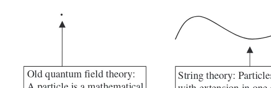
From the commutation relations and from the form of the fi elds (i.e., the creation and annihilation operators) you might glean that particle interactions take place at specifi c, individual points in space-time. This is important because it means that particle interactions take place over zero distance. Particles in quantum fi eld theory are point particles represented mathematically as located at a single point. This is illustrated schematically in Fig. 1.1.
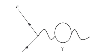
Now, calculations in quantum fi eld theory can be done using a perturbative expansion. Each term in the expansion describes a possible particle interaction and it can be represented graphically using a Feynman diagram. For example, in Fig. 1.2, we see two electrons scattering off each other.
The Feynman diagram in Fig. 1.2 represents the lowest-order term in the series describing the amplitude for the process to occur. Taking more terms in the series, we add diagrams with more complex internal interactions that have the same
Two particles come in to interact
The interaction occurs at a single point in space-time
Figure 1.1 In particle physics, interactions occur at a single point.
e
e e
e
γ
initial and fi nal states. For example, the exchanged photon might turn into an electron-positron pair, which subsequently decays into another photon. This is illustrated in Fig. 1.3.
Interior processes like that shown in Fig. 1.3 are called virtual. This is because they do not appear as initial or fi nal states. To fi nd the actual amplitude for a given process to occur, we need to draw Feynman diagrams for every possible virtual process, that is, take all the terms in the series. In practice we can take only as many terms as we need to get the accuracy desired in our calculations.
This type of procedure works well in the electromagnetic, weak, and strong interactions. However, the overall procedure has some big problems and they cannot be dealt with when gravity is involved. The problem comes down to the fact that interactions occur at a single space-time point. This leads to infi nite results in calculations (aptly called infi nities). Technically speaking, the calculation of a given amplitude which includes all virtual processes involves an integral over all possible values of momentum. This can be described by a loop integral that can be written in the form
I ∼
∫
p4J−8d pD (1.8)Here p is momentum, J is the spin of the particle, and D, which is seen in the integration measure, is the dimension of space-time. Now consider the quantity
λ =4J+ −D 8 (1.9)
If the momentum p→ ∞ and
λ <0
e e
e
e
γ
then I in Eq. (1.8) is fi nite and calculations give answers that make sense. On the other hand, if the momentum p→⬁but
λ >0
the integral in Eq. (1.8) diverges. This leads to infi nities in calculations. Now if I→⬁ but does so slowly, then a mathematical technique called renormalization can be used to get fi nite results from calculations. Such is the case when working with established theories like quantum electrodynamics.
The Standard Model
In its fi nished form, the theoretical framework that describes known particle interactions with quantum fi eld theory is called the standard model. In the standard model, there are three basic types of particle interactions. These are
• Electromagnetic
• Weak
• Strong (nuclear)
There are two basic types of particles in the standard model. These are
• Spin-1 gauge bosons that transmit particle interactions (they “carry” the force). These include the photon (electromagnetic interactions), W± and Z (weak interactions), and gluons (strong interactions).
• Matter is made out of spin-1/2 fermions, such as electrons.
In addition, the standard model requires the introduction of a spin-0 particle called the Higgs boson. Particles interact with the associated Higgs fi eld, and this interaction gives particles their mass.
Quantizing the Gravitational Field
a spin-2 boson, and so naturally includes the quantum of gravity. Returning to Eq. (1.8), if we letJ =2 and consider space-time as we know itD=4, then
4J− +8 D=4 2( )− + =8 4 4 So in the case of the graviton,
p4J−8→ p0=1 and
I ∼
∫
d p4 →⬁when integrated over all momenta. This means that gravity cannot be renormalized in the way that a theory like quantum electrodynamics can, because it diverges like p4. In contrast, consider quantum electrodynamics. The spin of the photon is 1, so
4J− +8 D=4 1( )− + =8 4 0 and the loop integral goes as
I ∼ p4J−8d pD p d p−4 4
∫
=∫
⇒Goes like
≈ p0=1
This tells us that incorporating gravity into the standard quantum fi eld theory framework is an extremely problematic enterprise. The bottom line is nobody really had any idea how to do it for a very long time.
String theory gets rid of this problem by getting rid of particle interactions that occur at a single point. Take a look at the uncertainty principle
∆ ∆x p∼
interactions (zero distance) imply infi nite momentum. This leads to divergent loop integrals, and infi nities in calculations.
So in string theory, we replace a point particle by a one-dimensional string. This is illustrated in Fig. 1.4.
Some Basic Analysis in String Theory
In string theory, we don’t go all the way to ∆ →x 0 but instead cut it off at some small, but nonzero value. This means that there will be an upper limit to momentum and hence ∆ /p→ ∞. Instead momentum goes to a large, but fi nite value and the loop integral divergences can be gotten rid of.
If we have a cutoff defi ned by the length of a string, then the uncertainty relations must be modifi ed. It is found that in a string theory uncertainty in position∆xis approximately given by
∆ =
∆ + ′ ∆
x p
p
α (1.10)
A new term has been introduced into the uncertainty relation, α′ ∆( p/ )which can serve to fi x a minimum distance that exists in the theory. The parameter α′is related to the string tension TS as
′ = α
π
1
2 TS (1.11)
The minimum distance scale we can see in string theory is given by
xmin∼2 α′ (1.12)
Old quantum field theory: A particle is a mathematical point, with no extension
.
String theory: Particles are strings, with extension in one dimension. This gets rid of infinities
So if α′ ≠0 , then the problems that result from pointlike interactions are avoided because they cannot take place. Interactions are spread out and infi nities are avoided.
String theory proposes to be a unifi ed theory of physics. That is, it is supposed to be the most fundamental theory that describes all particle interactions (known and perhaps currently unknown), particle types, and gravity. We can gain some insight into the unifi cation of all forces into a single framework by building up quantities from the fundamental constants in the theory.
If you have studied quantum fi eld theory then you know that a dimensionless constant called the fi ne structure constant can be constructed out of e, , and c where e is the charge of the electron, is Planck’s constant, and c is the speed of light. The fi ne structure constantαgives us a measure of the strength of the electromagnetic fi eld (through the coupling constant). It is given by
α
π
EM= ≈ <
e c
2
4
1
137 1 (1.13)
The fact that αEM <1 is what makes perturbation theory possible, since we can expand a quantity in powers of αEMto obtain approximate answers.
A similar procedure can be applied to gravity. We consider the gravitational force because it is the only force not described in a unifi ed framework based on quantum theory. The other known forces, the electromagnetic, the weak, and the strong forces are described by the standard model, while gravity sits on the sidelines relegated to the second string classical team. The constants important in gravitational interactions include Newton’s gravitational constant G, the speed of light c, and if we are talking about a quantum theory of gravity, then we need to include Planck’s constant . Two fundamental quantities can be derived using these constants, a length and a mass. This tells us the distance and energy scales over which quantum gravity will start to become important.
First let’s consider the length, which is aptly called the Planck length. It is given by
l G
c p=
−
∼
3
35
10 m (1.14)
This is one very small distance. For comparison, the dimension of a typical atomic nucleus is
lnucleus∼10−15 m
which is bigger than the Planck length by a factor of 1020! This means that quantum
gravitational effects can (naively at least) be expected to take place over very small distance scales. To probe such small distance scales, you need very high energies. This is confi rmed by computing the Planck mass, which turns out to be given by
M
Gc p=
−
∼108 kg (1.15)
While this is a small value to what might be measured when considering your waistline, it’s pretty large compared to the masses of the fundamental particles. This tells us, again, that high energies are needed to probe the realm of quantum gravity. The Planck mass also turns out to be the mass of a black hole where its Schwarzschild radius is the same as its Compton wavelength, suggesting that this is a length scale at which quantum gravitational effects become signifi cant.
Next we can form a Planck time. This is given by
t l
c p
p
= ∼10−44 s (1.16)
This is a small time interval indeed. So if you think quantum gravity, think small distances, small time intervals, and large energies. At these high energies gravity becomes strong. To see how this works think about the following. In a freshman physics course you learn that the electromagnetic force is something like 1040times
as strong as the gravitational interaction. But at the high energies we are describing, where quantum gravity becomes important, the strength of gravitational interactions is comparable to that of the other forces—gravity becomes strong and hence is important in particle interactions. Since the particle accelerators that are currently in existence (or that can even be dreamed up) probe energies that fall on a much smaller scale, gravity can be considered to be extremely weak at presently accessible energies.
String Theory Overview
Strings can be open (Fig. 1.5) or closed (Fig. 1.6), the latter meaning that the ends are connected.
Excitations of the string give different fundamental particles. As a particle moves through time, it traces out a world line. As a string moves through space-time, it traces out a worldsheet (see Fig. 1.7), which is a surface in space-time parameterized by ( , )σ τ . A mappingxµ( , ) maps a worldsheet coordinate τ σ
( , )σ τ to the space-time coordinate x.
So, in the world according to string theory, the fundamental objects are tiny strings with a length on the order of the Planck scale (10−33 cm). Like any string,
Figure 1.5 Fundamental particles are extended one-dimensional objects called strings.
Figure 1.6 A closed string has no loose ends.
x t
Schematic representation of a string moving through space-time, it is represented by a worldsheet (a tube for a closed string)
x t
A particle moving through space-time has a world line
Figure 1.7 A comparison of a worldsheet for a closed string and a world line for a point particle. The space-time coordinates of the world line are parameterized asxµ=xµ( )τ , while the space-time coordinates of the worldsheet are parameterized
these fundamental strings can vibrate and vibrations at different resonant frequencies (excitations of the string) give rise to particles with different properties. For a particle with spin J and mass mJ, the mass and spin of the particle are related to the string tension through α′as
J = ′α mJ2 (1.17)
Think of a vibrating string having different modes in the way that a violin string can vibrate at different frequencies. Instead of having a plethora of “fundamental particles” with mysterious origin, there is only one fundamental object—a string that vibrates with different modes giving the appearance that there are multiple fundamental objects. Each mode appears as a different particle, so one mode could be an electron, while another, different mode could be a quark.
It is possible for strings to split apart and to combine. Let’s focus on strings splitting apart. Suppose that a parent string is vibrating in a mode corresponding to particle A. It splits in two, with resulting daughter strings vibrating in modes corresponding to particles B and C respectively. This process of splitting corresponds to the particle decay:
A→ +B C
Conversely, strings can join up as well, combining to form a single string. This is a process that until now we have thought of as particle absorption. So processes that seemed more on the mysterious side, such as particle decay, are explained with a simple conceptual framework.
TYPES OF STRING THEORIES
There appear to be fi ve different types of string theory, but it has been shown that they are different ways of looking at the same theory, with the different types related by dualities. The fi ve basic types are
• Bosonic string theory This is a formulation of string theory that only has bosons. There is no supersymmetry, and since there are no fermions in the theory it cannot describe matter. So it is really just a toy theory. It includes both open and closed strings and it requires 26 space-time dimensions for consistency.
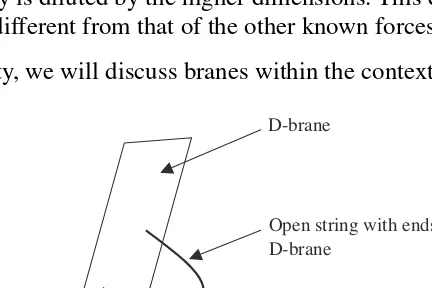
• Type II-A string theory This version of string theory also includes supersymmetry, and open and closed strings. Open strings in type II-A string theory have their ends attached to higher-dimensional objects called D-Branes. Fermions in this theory are not chiral.
• Type II-B string theory Like type II-A string theory, but it has chiral fermions.
• Heterotic string theory Includes supersymmetry and only allows closed strings. Has a gauge group called E8×E8. The left- and right-moving modes on the string actually require different numbers of space-time dimensions (10 and 26). We will see later that there are actually two heterotic string theories.
M-THEORY
All these string theories might seem confusing, and make the whole enterprise seem like a stab in the dark. However, as we go through the book we will learn about the different dualities that connect the different types of string theories. These go by the names of S duality and T duality.
Since these dualities exist, there has been speculation that there is an underlying, more fundamental theory. It does by the odd name of M-theory but “M” does not really have any agreed upon or specifi c meaning (perhaps mother of all theories). One concept in M-theory is that the space-time manifold (i.e., its structure) is not assumed a priori but rather emerges from the vacuum.
One concrete manifestation of M-theory is based on matrix mechanics, the kind you are used to from ordinary quantum mechanics. In this context “M” really means something, and we call it matrix theory. In this theory, if we compactify (i.e., make really tiny) n spatial dimensions on a torus, we get out a dual matrix theory that is just an ordinary quantum fi eld theory in n + 1 space-time dimensions.
D-BRANES
A D-brane, mentioned in our discussion of string theory types, is an extension of the common sense notion of a membrane, which is a two-dimensional brane or 2-brane. A string can be though of as a one-dimensional brane or 1-brane. So a p-brane is an object with p spatial dimensions.
of gravity, are not attached to D-branes. They can travel or “leak off” a D-brane, so we don’t see as many of them. This explains what until now has been a great mystery, why electromagnetism (and the other known forces) is so much stronger than gravity.
So this picture of the universe has a three-dimensional brane (or 3D-brane) embedded in a higher-dimensional space-time called the bulk. Since we interact with the physical world primarily through electromagnetic forces (light, chemical reactions, etc.), which are mediated by particles that are really strings stuck to the brane, we experience the world as having three spatial dimensions. Gravity is mediated by strings that can leave the brane and travel off into the bulk, so we see it as a much weaker force. If we could probe the bulk somehow, we would see that gravity is actually comparable in strength.
HIGHER DIMENSIONS
We live in a world with three spatial dimensions. In a nutshell this means that there are three distinct directions through which movement is possible: up-down, left-right, and forward-backward. In addition, we have the fl ow of time (forward only as far as we know). Mathematically, this gives us the relativistic description of coordinates ( , , , )x y z t .
It is possible to imagine a world where one of the spatial directions or dimensions have been removed (say up-down). Such a two-dimensional world was described by Edward Abbott in his classic Flatland. What if instead, we added dimensions? This idea is actually pretty useful in physics, because it provides a pathway toward unifying different physical theories. This kind of thinking was originally put forward by two physicists named Kaluza and Klein in the 1920s. Their idea was to bring gravity and electromagnetism into a single theoretical framework by imagining that these two theories were four-dimensional limits of a fi ve-dimensional supertheory. This idea did not work out, because back then people did not know about quantum fi eld theory and so did not have a complete picture of particle interactions, and did not know that the fully correct description of electromagnetic interactions is provided by quantum electrodynamics. But this idea has a lot of appeal and reemerged in string theory.
String theory requires the existence of extra spatial dimensions for technical reasons that we will discuss in later chapters. An interesting side effect of these extra dimensions is that another mystery of particle physics is done away with. Experimentalists have worked out that there are three families of particles. For example, when considering leptons, there is the electron and its corresponding neutrino. But there are also the “heavy electrons” known as the muon and the tau, together with their corresponding neutrinos, that are really just duplicates of the electron. The same situation exists for the quarks. Why are there three particle families? And why are there the types of particle interactions that we see? It turns out that higher spatial dimensions together with string theory may provide an answer.
The way that you compactify the extra dimensions (the topology) determines the numbers and types of particles seen in the universe. In string theory this results from the way that the strings can wrap around the compactifi ed dimensions, determining what vibrational modes are possible in the string and hence what types of particles are possible.
One important compactifi ed manifold that we will see is called the Calabi-Yau manifold. A Calabi-Yau manifold that compactifi es six spatial dimensions and leaves three spatial dimensions “macroscopic” plus time gives a ten-dimensional universe as required by most of the string theories. A key aspect of Calabi-Yau manifolds is that they break symmetries. Thus another mystery of particle physics is explained, so-called spontaneous symmetry breaking (see Quantum Field Theory Demystifi ed for a description of symmetry breaking).
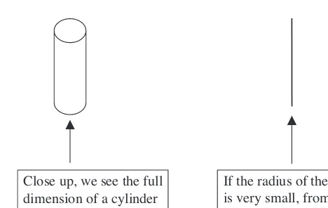
Close up, we see the full dimension of a cylinder
If the radius of the cylinder is very small, from far away the cylinder appears one-dimensional, as a line
Figure 1.8 Compactifi cation explains why we may not be aware of extra spatial dimensions even if they exist. If the radius of a cylinder is very
Summary
Quantum mechanics and general relativity were the major developments in theoretical physics in the twentieth century. Unifying them into a single theoretical framework has proven extremely challenging, if not impossible. This is because the resulting quantum theories are plagued by infi nities that result from the fact that interactions take place at a single mathematical point (zero distance scale). By spreading out the interactions, string theory offers the hope of developing not only a unifi ed theory of particle physics, but a fi nite theory of quantum gravity.
Quiz
1. If λ =4J+ − >D 8 0and p→⬁ then (a) the loop integral is convergent. (b) the loop integral diverges.
(c) the loop integral can be calculated, but the results are meaningless. 2. The scale of the Planck length and Planck mass tell us that quantum gravity
(a) operates on small-distance and high-energy scales. (b) is nonsensical.
(c) operates on small-distance and small-energy scales. (d) operates on large-distance and small-energy scales.
3. Perturbation theory is possible in quantum electrodynamics because (a) αEM >1
(b) αEM=1
(c) αEM <1
(d) Perturbation theory is not possible in quantum electrodynamics 4. The quantum uncertainty relations are modifi ed in string theory as
(a) ∆
∆ + ∆
x p
p ∼
(b) ∆
∆ + ′ ∆
x p
p
∼ α
(c) ∆
∆ − ′ ∆
x p
p
∼ α
(d) ∆ ′∆
x
p ∼
5. The minimum distance scale in string theory is about
(a) xmin∼ 1 2 α′
(b) xmin∼2 TS
(c) xmin∼0
(d) x
TS
min=
2
π
6. The topology of compactifi ed dimensions
(a) determines the types of particles seen in the universe. (b) has no impact on particle interactions.
(c) restores symmetries in quantum fi eld theories. 7. Heterotic string theory has the gauge group
(a) E6×E6 (b) SU(32) (c) E8×E8 (d) SO( )16
8. String theory explains the difference between electromagnetism and gravity as (a) String theory provides the unifi cation energy of gravity and electromagnetism. (b) Gravitons are not connected to the brane, so can leak off into the bulk
making gravity appear much weaker than electromagnetism. (c) Photons leak off into the bulk, making electromagnetic phenomena
more prominent.
9. Bosonic string theory is not realisitic because (a) it includes 26 space-time dimensions.
(b) it does not allow Calabi-Yau compactifi cation.
(c) it does not include fermions, so cannot describe matter. (d) it lacks a E8×E8symmetry group.
10. In string theory particle decay is explained by
(a) a string splitting apart into multiple daughter strings. (b) it remains poorly understood.
The Classical String I:
Equations of Motion
When you studied classical mechanics and quantum fi eld theory, you learned about the action and deriving the equations of motion from the Euler-Lagrange equations. This can be done in the case of the string, and it can be done relativistically. If we are going to consider a unifi ed theory of physics, this is a good place to start— ensuring that we understand how to describe the dynamics of strings in a manner that is fully consistent with relativity before moving on to introduce the quantum theory.
When we quantize our strings, our fi rst foray into a fully relativistic, quantum theory will be an instructive but unrealistic case, the bosonic string. As the name implies, we are going to look at a theory consisting exclusively of bosons—that is, states with integral spin. We know that this cannot be a realistic theory because in
the actual universe while force-carrying particles are indeed bosons, fundamental matter particles (like electrons) have half-integral spin, that is, they are fermions. So a theory that describes a world consisting entirely of bosons does not describe the real universe.
Nonetheless, we start here because it is an easier way to approach string theory and we can learn the nuts and bolts in a slightly simpler context. We are going to approach bosonic strings in three steps. In this chapter, we will develop the theory of classical, relativistic strings starting with the action principle and deriving the equations of motion. In Chap. 3, we will learn about the stress-energy tensor and conserved currents, specifi cally conserved worldsheet currents. Finally, in the last chapter of this part of the book, we will quantize the strings using a procedure of fi rst quantization (i.e., fi rst quantization of point particles gives single-particle states). In the end you have a quantized relativistic theory.
To this end, we begin our journey into the world of classical relativistic point particle moving in space-time to illustrate the techniques used.
The Relativistic Point Particle
The task at hand is to describe the motion of a free (relativistic) point particle in space-time. One way to approach the problem is by using an action principle. Before we do that, let’s set up the arena in which the particle moves. Let its motion be defi ned with respect to space-time coordinates Xµ where X0 is the timelike coordinate (i.e., X0=ct) and Xi where i≠0 are the spacelike coordinates (say x, y, and z). While you are probably used to lowercase letters like xµ to represent coordinates, in string theory uppercase letters are used, so we will stick to that convention.
Anticipating the fact that string theory takes place in a higher-dimensional arena, rather than the usual one time dimension and three spatial dimensions we are used to, we consider motion in a D-dimensional space-time. There is one time dimension but now we allow for the possibility of d=D −1 spatial dimensions. We reserve 0 to index the time dimension hence our coordinates range over µ =0,. . .,d.
Now, the motion or trajectory of a particle is described such that the coordinates are parameterized by τ, which parameterizes the world-line of the particle. That is, this is the time given by a clock that is moving or carried along with the particle itself. We can emphasize this parameterization by writing the coordinates as functions of the proper time:
To describe distance measurements, we are going to need a metric, that is, a function which allows us to defi ne the distance between two points. Here we will stick with special relativity and use the fl at space Minkowski metric which is usually denoted by ηµν. You may recall that the time and spatial components of the metric have different sign; the choice used is referred to as the signature of the metric. In string theory, it is convenient to place the negative sign with the time component, so in the case of d=3 spatial dimensions we can write the Minkowski metric as a matrix
ηµν = − ⎛
⎝ ⎜ ⎜ ⎜ ⎜
⎞
⎠ ⎟ ⎟ ⎟ ⎟
1 0 0 0 0 1 0 0 0 0 1 0 0 0 0 1
(2.2)
More compactly, we can write ηµν = − + + +( , , , ). Generalizing to D-dimensional Minkowski space-time, we simply associate a plus sign with products of spatial coordinates. So the Lorentz invariant length squared of a vector is
(Xµ)2 =ηµνX Xµ ν = −(X0 2) +(X1 2) + +(Xd)2 (2.3) Infi nitesimal lengths or distances are described by
ds2 = −ηµνdX dXµ ν =(dX0 2) −(dX1 2) − (dXd) (2.4)2 We include the minus sign out in front of the metric in Eq. (2.4) to ensure that
ds= −ηµνdX dXµ ν is real for timelike trajectories. With these notations in hand, we are ready to describe the trajectory of a free relativistic particle using the action principle.
The action principle tells us that the relativistic motion of a free particle is proportional to the invariant length of the particles trajectory. That is,
S= −α
∫
ds (2.5) First let’s fi gure out what the constant of proportionality is.EXAMPLE 2.1
Given that the action of a free, non-relativistic particle is S0= dt 1 2mv2
∫
( / ) , whereSOLUTION
For simplicity, we consider motion in one spatial dimension. Now
S ds
dt dx
dt dx
dt
dt
= −
= − −
= − −
= − −
∫
∫
∫
α α α α
2 2
2 2
1
1 v2
∫
Now recall the binomial theorem. This tells us that
1 1 1
2
± ≈ ±x x
Hence,
1 1 1
2
2 2
−v ≈ − v
Therefore
S dt v
dt v dt dt v
= − −
≈ − ⎛⎝⎜ − ⎞⎠⎟ = − +
∫
∫
∫
α
α α α
1
1 1
2
1 2
2
2 2
∫∫
Comparison of the second term in this expression with S0=
∫
dt( / )1 2 mv2 tells us that α must be the mass of the particle.We can also determine the units of α and deduce that it is the mass of the particle from dimensional analysis. First, what are the units of action? Recall from your studies of quantum theory that the units of action from Planck’s constant are mass times length squared per time:
[ ]= ML
T
2
Now let’s look at S= −α
∫
ds. From the integral, we have length L, so we have MLT L
2
=[ ]α So it must be the case that
[ ]α = ML T
We can obtain this result using the mass of the particle together with the speed of light c, which is of course a length over time. That is,
α α
= ⇒ =
m c ML
T [ ]
In units where c= =1, which are commonly used in particle physics and string theory, the action is dimensionless. Hence mass is inverse length and
α α
= ⇒ = =
m
M L
[ ] 1 (2.7)
Now let’s see how to write down the action and obtain the equations of motion from it. We start with the defi nition of infi nitesimal length given in Eq. (2.4). This gives the action as
S= −m
∫
−ηµνdX dXµ ν (2.8)Let’s rewrite the integrand:
− = − ⎛
⎝⎜ ⎞ ⎠⎟ = −
η η τ
τ τ η
µν µ ν µν µ ν
µν µ
dX dX d
d dX dX
d dX
d
2
ττ τ τ η
ν
µν µ ν
dX
This allows us to write the action in the form
S= −m d
∫
τ −ηµνX Xµ ν (2.9)This action is a nice compact form that allows us to derive the equations of motion. As you recall from your studies of classical mechanics or quantum fi eld theory, the quantity in the integrand is called the lagrangian:
L= −m −ηµνX Xµ ν= −m −X2
There are two problems with the action so far developed in Eq. (2.9). First, think about what happens in the case of a massless particle. Setting m=0 leaves us with S→0 and so there is nothing to vary to obtain the equations of motion. So this action isn’t very helpful in the case of a massless particle. Also, it turns out that quantization is not easy when we have a square root in the action. For these reasons, we introduce an auxiliary fi eld that we will denote a( )τ and consider the lagrangian
L aX
m a
= 1 −
2 2
2 2
We can use this to defi ne an alternative expression for the action
′ = ⎛ − ⎝⎜
⎞ ⎠⎟
∫
S d
aX m a
1 2
1 2 2
τ (2.10)
We can vary this action to fi nd an equation of motion for the auxiliary fi eld a( )τ . We fi nd
δ δ τ
τ δ
′ = ⎛ −
⎝⎜
⎞ ⎠⎟
= ⎛
⎝⎜ ⎞ ⎠⎟
∫
∫
S d
aX m a
d
a X
1 2
1
1 2
1
2 2
2−−
⎛ ⎝⎜
⎞ ⎠⎟
= ⎛− −
⎝⎜
⎞ ⎠⎟
∫
δ
τ
(m a)
d
a X m
2
2
2 2
1 2
Now we set δ ′ =S 0. Since this means that the integrand must be 0, we obtain the equation − − = ⇒ + = 1 0 0 2 2 2
2 2 2
a X m
X m a
This is the equation of motion for the auxiliary fi eld. From this we fi nd an expression for the auxiliary fi eld given by
a X
m
= − 22 (2.11)
Using Eq. (2.11), we can show that the action in Eq. (2.10) is equivalent to Eq. (2.8), which we do in the next example.
EXAMPLE 2.2
Show that if a= −( X2/m2 1 2)/ , the action ′ = −
∫
S 1 2/ dτ[( / )1 a X2 m a2 ] can be recast
in the form S= −m
∫
−ηµνdX dXµ ν.SOLUTION
Let’s start by recalling that X2=ηµνX Xµ ν. So we can rewrite the action S′ in the following way: ′ = ⎛ − ⎝⎜ ⎞ ⎠⎟ = − − −
∫
∫
S daX m a
d m
X X m
1 2 1 1 2 2 2 2 2 2 2 τ
τ XX
m
d m
X X m X
d 2 2 2 2 2 2 1 2 1 2 ⎛ ⎝ ⎜ ⎞ ⎠ ⎟ = ⎛ − − − ⎝ ⎜ ⎞ ⎠ ⎟ =
∫
τ τ∫∫
⎛ − − − ⎝ ⎜ ⎞ ⎠ ⎟ mX X m X X
2 2
2 η
Now, let’s use a simple algebraic trick to rewrite the fi rst term. Remember from complex variables that i2= −1. This means that
−
= − − −
= − −
= − −
m
X X
m
X X
m
X i X
2 2
2
2 2
2
2 2
2 2
1 1
( )( )
m m
X i X
m i X
m i X
2 2
4 4
2 4 2
4 2
= − − = − −
But i4 = +1, and so −m −i X4 2 = −m −X2 = −m −ηµνX Xµ ν. Therefore the action is
′ = ⎛ − − − ⎝
⎜ ⎞
⎠ ⎟
= −
∫
∫
S d m
X X m X X
d m
1 2
1 2
2 2
2
τ η
τ
µν µ ν
ηη η
τ η
µν µ ν µν µ ν
µν µ ν
X X m X X
m d X X
− −
(
)
= −
∫
(
−)
=SSThis demonstrates that the two actions are equivalent.
Strings in Space-Time
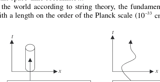
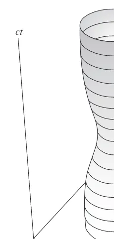
motion can be described by saying that a point particle (zero-dimensional) sweeps out a path or line in space-time (one dimension) that we call the world-line. A string, unlike a point particle, has some extension in one dimension, so it’s a one-dimensional object. As it moves, the string (one-one-dimensional) sweeps out a two-dimensional surface in space-time that scientists call a worldsheet. For example, imagine a closed loop of string moving through space-time. The worldsheet in this case will be a tube, as shown in Fig. 2.1.
We can summarize this in the following way:
• The path of a point particle is a line in space-time. A line can be parameterized by a single parameter, which is the proper time.
• As a string moves through space-time it sweeps out a two-dimensional surface called a worldsheet. Since the worldsheet is two-dimensional, we need two parameters, which we can generally denote by ξ1 andξ2.
Locally the coordinates ξ1andξ2 can be thought of as coordinates on the worldsheet. Or, another way to look at this is to parameterize the worldsheet, we need to account for proper time and the spatial extension of the string. So, the fi rst parameter
ct
is once again the proper time τ, and the second parameter, which is related to the length along the string, is denoted by σ:
ξ1=τ ξ2=σ
Coordinates on the worldsheet ( , )τ σ are mapped onto space-time by the functions (called the string coordinates)
Xµ( , ) (2.12)τ σ
So time and spatial position on the string are mapped onto the spatial coordinates in (d + 1) dimensional space-time as
{X0( , ),τ σ X1( , ),τ σ …,Xd( , )}τ σ
Now, we need to write down the action for the string which will generalize Eq. (2.8) to our new higher-dimensional world, that is, to the case of the worldsheet. This is done in the following way. Recall that the action of a point particle is proportional to the length of its world-line [Eq. (2.5)]. We just noted that a string sweeps out a two-dimensional worldsheet in space-time. This tells us that if we are going to generalize the notion of the action of a point particle, we might expect that the action of a string is proportional to the surface area of the worldsheet. This is in fact the case. Anticipating that the constant of proportionality will turn out to be the string tension, we can write this action as
S= −T dA
∫
(2.13)where dA is a differential element of area on the worldsheet. To fi nd the form of dA, we start by considering a differential line element ds2 and introduce coordinates on the worldsheet as ξ1=τ andξ2=σ. Doing a little algebra we have
ds dX dX
X X
d d
2= −
= − ∂ ∂
∂ ∂ η
η
ξ ξ ξ ξ
µν µ ν
µν µ
α ν
β
α β
This allows us to defi ne an induced metric on the worldsheet. This is given by
γ η
ξ ξ
αβ µν µ
α ν
β
= ∂ ∂
∂ ∂
X X
This metric determines distances on the worldsheet. We say that this metric is induced because it includes the metric of the background space-time in its defi nition
(we are taking space-time to be fl at, so are using ηµν). That is to say, on the surface of the worldsheet, there is a new measure of distance, but that measure of distance is determined by the background space-time through its metric (which in general, is not ηµν). Proceeding, we now have
ds2 =γαβdξ ξαd β
Using the notations
Xµ X X X
µ
µ µ
τ σ
=∂
∂ ′ = ∂∂
We can write the components of the induced metric (for the case of fl at space-time) as
γ η
τ τ γ η
σ τ
ττ µν
µ ν
στ µν
µ ν
= ∂ ∂
∂ ∂ = = ∂
∂ ∂
∂ = ⋅ ′
X X
X
X X
X
2
X
X X X
X X
X
= = ∂ ∂
∂ ∂ = ∂
∂ ∂
∂ = ′
γ η
τ σ γ η
σ σ
τσ µν
µ ν
σσ µν
µ ν
2
(2.15)
Using Eq. (2.15), we can write the induced metric as a matrix in ( ,τ σ) space
γαβ = ⋅ ′ ⋅ ′ ′ ⎛
⎝⎜
⎞ ⎠⎟
X X X<