Light scattering by penetrable convex polygons

(1)

University of Reading

School of Mathematical and Physical Sciences

Light scattering by penetrable

convex polygons

Samuel Groth

August 2011

This dissertation is for a joint MSc in the Departments of Mathematics & Meteorology and

(2)

Abstract

This thesis concerns the problem of time-harmonic electromagnetic scattering by a penetrable two-dimensional convex polygon. This problem finds applications in many

areas such as radar imaging, telecommunications and, of specific interest in this study, the scattering properties of atmospheric ice crystals. Standard numerical methods for

such problems have a computational cost which grows linearly with the frequency of the incident wave. High frequency asymptotic approaches such as ray tracing do not

suffer from this problem, however give poor accuracy at low frequencies. This thesis analyses the behaviour of optical diffraction to further the progress toward producing

an approximation method for this problem which is applicable at all frequencies of the incident wave. A ray tracing algorithm is presented and the approximation produced

is subtracted from that of a standard boundary element method. This difference is identified as being due to diffraction and is experimented with in order to describe

(3)

Acknowledgements

I would like to thank my supervisors Dr. Stephen Langdon and Dr. David Hewett for their help, encouragement and direction throughout this project. I would also like to

thank the Natural Environmental Research Council for their financial support which allowed me to take part in this course.

(4)

Declaration

I confirm that this is my own work and the use of all material from other sources has been properly and fully acknowledged.

Signed...

(5)

List of Figures

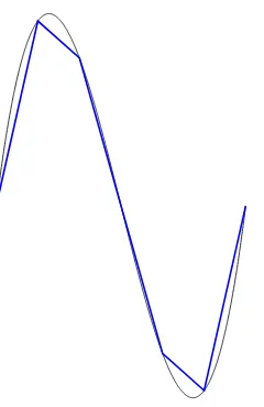
1.1 Wave approximated by piecewise polynomials. Here the polynomials are

linear for clarity, however they may also be quadratic, cubic, etc. . . 2

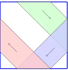
1.2 Ray tracing inside the polygon. Note that the transmitted rays have not been included in this diagram. . . 3

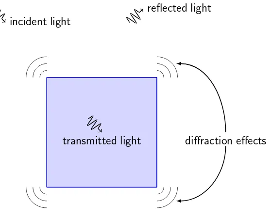
1.3 Reflection, transmission and diffraction of light. . . 4

2.1 Range of ice crystal sizes over which different methods are applicable. 7 4.1 Polygon notation. . . 20

4.2 Plots showing the approximation to the field produced by the boundary element method. . . 29

5.1 Ray tracing. . . 31

5.2 Refraction and reflection of light at the interface y= 0 . . . 33

5.3 Coordinate shift and rotation. . . 38

5.4 Ray tracing inside the polygon. Note that the transmitted rays have not been included in this diagram. . . 41

5.5 Setup for the square with P1 = (π, π),P2 = (−π, π),P3 = (−π,−π) and P4 = (π,₋π). . . 43

(8)

viii LIST OF FIGURES

5.6 Ray tracing approximation with M = 50 of the electric field on the

boundary of the square ice crystal in Figure 5.5 which is being irradiated by light with wavenumber k = 5, amplitude A = 1 and direction di = (1,₋1). . . 44

5.7 Ray tracing approximation of the electric field on the boundary of the square crystal in Figure 5.5 which is being irradiated by light with

wavenumber k = 5, amplitude A = 1 and direction di = (1,₋1). Each subsequent plot shows the field after considering one more

reflec-tion/transmission, so we go from M = 1 to M = 4. . . 45

6.1 Plots showing the logarithm of errorM against the number of

reflec-tions/transmissions M. . . 55

6.2 Decay of errorM for square obstacle with refractive index m2 = 2 and

incident light wavenumber k= 10. . . 56

6.3 Error decay of geometric series versus error decay of RT . . . 56

6.4 Comparisons between outputs of BEM and RTA for square scatterer irradiated by light with wavenumber k = 10. . . 57

6.5 Absolute values of the real and imaginary components of ud on the

boundary of the square with incident light of wavenumber k = 30. . . . 58

6.6 How diffracted fields are reflected within the shape. The dashed lines

represent the beam edges as predicted by ray theory. . . 59

(9)

Chapter 1 Introduction

In this thesis we study the scattering of time-harmonic electromagnetic waves in two dimensions by a penetrable convex polygon. In particular, we focus on the problem of

light scattered by a 2D ice crystal. We specify that the crystal shape must be convex, i.e. all exterior angles greater than 180◦_{, so that the scattered light is not re-reflected}

by the external boundary at any point. Of course, since the crystal is penetrable (transparent), the light will be transmitted into the interior and undergo infinitely

many internal reflections. At each of these reflections part of the wave’s energy is reflected back into the crystal and the rest is transmitted out (except for the case of

total internal reflection where all the wave’s energy is reflected). Each time part of the wave’s energy is transmitted out of the crystal, this contributes to the exterior

‘scattered’ electromagnetic field. The aim of the scattering problem is to determine this scattered field which, when combined with the incident electromagnetic field, gives

us the pattern of light outside the crystal.

Since no analytic solution for scattering by a penetrable polygon exists, we must

turn to numerical methods to provide an accurate approximation. Some of the stan-dard approaches are boundary and finite element methods in which the scattered field

is approximated using piecewise polynomials [6]. Figure 1.1 shows one wavelength

(10)

2 CHAPTER 1. INTRODUCTION

Figure 1.1: Wave approximated by piecewise polynomials. Here the polynomials are

linear for clarity, however they may also be quadratic, cubic, etc.

proximated by several polynomials of degree 1. In general we may use polynomials of

degreen, i.e. of the form p=a0+a1x+a2x2₊_...₊_a

nxn, and we say each polynomial

has (n+ 1) degrees of freedom. So, for example, using 5 polynomials of degree 1 to

approximate a wavelength is equivalent to using 2 polynomials of degree 4 (from a com-putational cost point of view), since they both result in 10 degrees of freedom. In order

to resolve the wave solution well we must take a fixed number of degrees of freedom P

for each wavelength, with the standard practice in the literature being to takeP = 10

(see e.g. [6] or [15]). Naturally, if we shorten the wavelength of the incident light, there are more wavelengths that will fit across our scatterer, hence the number of degrees of

freedom of the problem increases. The same is also true if we keep the wavelength fixed but increase the size of the scatterer.

To consider this more precisely, let D be the diameter of the smallest circle that

will enclose the ice crystal and write k = 2π/λ where λ is the wavelength, so that

k is the wavenumber. Then the total number of degrees of freedom d required to

represent the solution well on the boundary is proportional to kD. This means that these standard numerical methods become very computationally demanding for light of

(11)

3

a quantity called the scale parameter defined as X = kD/2π = D/λ; this represents

the number of wavelengths that fit across the diameter of the crystal. Then we can say that d_∝X for these numerical methods.

Now, there are alternative methods for solving this problem whose efficiency does

not scale withX. One of these, namely ‘ray tracing’, is the main topic of this thesis. Ray tracing is an approach which tracks the beams of light as they are reflected around inside

the crystal (see Figure 1.2). This technique is purely geometrical in that it calculates the beams’ reflected and transmitted directions and amplitudes based on the geometry

of the shape and the direction of the incident light. If we consider enough reflections and transmissions, we can build up a representation of the scattered electromagnetic

field. Since this method is geometrical, its computational cost is independent of the size parameter X. So what’s wrong with it?

Figure 1.2: Ray tracing inside the polygon. Note that the transmitted rays have not been included in this diagram.

The drawback of ray tracing is that it is an asymptotic method, which is valid only in the limit asX _{→ ∞}. From a mathematical point of view, this means that for a fixed

X we cannot achieve arbitrary accuracy using a ray tracing method. From a physical point of view, the main deficiency of the method is that, in its simplest form, it does not

account for the phenomenon of light ‘bending’ around corners, i.e. optical diffraction, a basic depiction of which is shown in Figure 1.3. We note here that higher-order ray

(12)

4 CHAPTER 1. INTRODUCTION

Geometric Theory of Diffraction [13]). However, their application to the transmission

problem has been limited due to the difficulty encountered in analysing the relevant ‘canonical’ scattering problems, such as the diffraction of a plane wave by an infinite

penetrable wedge (see [16]).

diffraction effects incident light

reflected light

transmitted light

Figure 1.3: Reflection, transmission and diffraction of light.

The effect of diffraction is expected to be negligible for large X, but for small or

moderate X it may be significant. In this thesis our aim is to examine the difference between the approximations obtained using a boundary element method (BEM) and

a ray tracing algorithm (RTA) in order to better understand the behaviour of the diffracted field in the transmission problem. The ultimate goal of this work would be

to develop a technique in which a RTA is used to evaluate the leading order behaviour (i.e. main features) of the scattered field and then a specially designed BEM is employed

to efficiently evaluate the additional field due to diffraction.

Now to give a brief outline of this thesis: we begin in Chapter 2 by mentioning an important application of light scattering by ice crystals to atmospheric science and by

(13)

5

in electromagnetism and the derivation of our fundamental governing equation, namely

the Helmholtz equation. It is shown that solving the scalar case - which is equivalent to an acoustic transmission problem - is sufficient. Then, in Chapter 4, we

reformu-late the Helmholtz equation as a boundary integral equation with the aid of Green’s Representation Theorem which sets us up to describe boundary element methods for

solving the scattering problem numerically. Chapter 5 describes the construction of a RTA including the derivations of important geometrical equations such as Snell’s Law

and the Fresnel equations.

We now come to the results section of the thesis. In Chapter 6 we compare the approximations given by a RTA, written by myself, and a BEM provided by David

Hewett. We also examine the convergence behaviour of the ray tracing solution. We conclude in Chapter 7 with an overview of the theory and results of the thesis and also

(14)

Chapter 2 Background and Motivation

Scattering theory attempts to understand how the propagation of acoustic and elec-tromagnetic waves is affected by obstacles and inhomogeneities. Areas in which this

theory finds applications include modelling radar, sonar, medical imaging and atmo-spheric particle scattering. The last example in this list is of particular interest in this

thesis, but more specifically we are interested in understanding the electromagnetic scattering properties of ice crystals found in the upper atmosphere.

Most of these ice crystals are found in cirrus clouds which generally form at altitudes

greater than 6 km and can permanently cover up to 30% of the Earth’s surface [3]. As a consequence, these clouds have a large influence on the Earth’s radiation budget

and as such are an important factor to consider when predicting climate change. At present the effect of cirrus clouds on the Earth’s climate is poorly understood due to

the difficulty in determining their reflection and transmission properties. Knowledge of

these properties would enable us to infer the optical thickness of cirrus clouds.

Optical thickness is a measure of transparency and tells us how much incident solar radiation is transmitted through the cloud. If a cloud is optically thin, then a

large amount of the incident sunlight will be transmitted (hence a small amount will be reflected back to space) and long-wave radiation emitted from the Earth will be

(15)

7

absorbed which leads to a warming at the Earth’s surface. If, however, a cloud is

optically thick, a larger amount of incident sunlight is reflected back into space than is transmitted towards the Earth, which leads to a cooling at the surface (for further

details see [2]).

The difficulty in understanding the scattering properties of these clouds stems from the fact that the constituent ice-crystals are mostly non-spherical, since no analytic

solution exists for such shapes. In fact, it has been observed from aircraft and satellite observations that the ice crystals come in a large array of shapes such as hexagonal

columns and plates, bullet-rosettes and hexagonal aggregates, the size of which can range from 1µm to 1000µm [11]. So the size parameter X can between 1 and 2500 for

visible light, which has a wavelengthλ in the range 390 nm to 750 nm.

A great deal of work has been done (see e.g. [18] and [19]) on tackling the problem

of light scattering by atmospheric ice crystals and indeed a large amount of success has been achieved. However, at present there exist separate groups of techniques which

are applicable for different ranges of X. As can be seen in Figure 2.1, numerical methods such as boundary and finite element methods and finite difference time domain

methods are only useful for relatively smallXdue to computational constraints, whereas geometrical optics methods such as ray tracing are accurate for large X. There is a

void between these two ranges ofX for which neither approach is of use.

Numerical methods

Hybrid methods?

Geometrical Optics

Figure 2.1: Range of ice crystal sizes over which different methods are applicable.

The prime motivation for this thesis is the desire to ‘bridge this gap’ by designing a method which is suitable for the values of X which currently cannot be modelled

(16)

8 CHAPTER 2. BACKGROUND AND MOTIVATION

that we would be able to obtain as accurate an approximation as we wished, for example

by increasing the resolution of the mesh or by taking more terms in the series. Such a feature is present in numerical methods, however geometrical optics techniques do not

have this advantage since they are fundamentally an asymptotic approximation and so will never resolve the effects of diffraction.

Another motivation for this work is the goal to develop one model which can be

applied for all values ofX, since we wish ultimately to simulate the scattering properties of an entire cloud of ice crystals with a range of sizes. To this end, Yang and Liou have

designed a novel geometric ray tracing model, to which the RTA created in this thesis is similar, which is highly accurate for large values of X but increasingly less accurate

as X decreases. Also, Silveira [17] has taken the X-independent Galerkin boundary element method of Chandler-Wilde and Langdon [6], which was designed for the sound

soft acoustic problem, and applied it to the transmission problem of concern here. Silveira’s approach is to incorporate diffraction but ignore reflections of the rays within

the interior of the obstacle. More precisely, the leading order behaviour on the sides in shadow is assumed to be negligible. The quality of the results from Silveira’s study

suggests that we must use a more sophisticated approach in ascertaining the leading order behaviour on the shadowed sides [17]. Note that by ‘shadowed sides’ we mean

those which are not lit by the incident light directly, i.e. the light must pass through the crystal to hit them.

In this thesis we take the first steps to improving upon Silveira’s attempt to extend the reach of numerical methods. Our approach will be to study the difference between

the leading order behaviour of the fieldul and the total fieldu. We term this difference

ud and write it explicitly as

ud=u−ul.

This is done by first supposing that ul can be determined by the RTA and that ud is

therefore due to diffraction effects. By studying ud and understanding its properties

(17)

9

hope in future studies to further the work of Chandler-Wilde and Langdon in [6] in

order to develop an X-independent numerical method for the transmission problem. This would constitute a major advance in the area of computational methods for

high-frequency scattering problems. Such a method would use a RTA to calculate the leading order behaviour, ul, and a specially designed BEM to calculate the extra field due to

(18)

Chapter 3 Electromagnetism

Light waves are the manifestation of perturbations in the electromagnetic field and, as such, any attempt to understand the scattering behaviour of light must begin with an

exposition of the theory of electromagnetism. We begin by stating the four fundamental equations first written down by James Clerk Maxwell in 1861 and see how they simplify

when considering light travelling through air and ice. We find that we may ignore one of the five vectors of electromagnetism since it is negligibly small in these two media.

In_§3.2 we consider the conditions that we require the electromagnetic vectors to satisfy on the boundary of the ice crystal. It is important to enforce such conditions because

Maxwell’s equations are only valid for media in which certain properties such as the dielectric constant – which we see in _§3.3 is analogous to the refractive index – are

continuous. It is well known that light refracts or ‘bends’ as it passes from air into ice because their respective refractive indices are different. Therefore we must impose

boundary conditions at the surface of the crystal to ensure that Maxwell’s equations hold here.

In _§3.3 we demonstrate that light travels as waves and, restricting our attention to time-harmonic waves, we derive our governing equation, that is Helmholtz’s equation.

Finally in_§3.4 we look at the 2D case which is relevent in this thesis and show that we

(19)

3.1. MAXWELL’S EQUATIONS 11

arrive at the scalar transmission problem, which is equivalent to the 2D acoustic case.

3.1 Maxwell’s Equations

In this section, and the following two, we follow the exposition of Born and Wolf [4]. The electric vectorEand the magnetic induction Btogether constitute the electromagnetic

field. To describe the effect of the field on matter we must introduce three further vectors: j the electric current density,D the electric displacement and Hthe magnetic

vector. The space and time derivatives of these five vectors are related via Maxwell’s equations1

∇ ×H₋ 1

cD˙ =

4π

c j, (3.1)

∇ ×E+1

cB˙ = 0, (3.2)

∇ ·D = 4πρ, (3.3)

∇ ·B = 0, (3.4)

whereρ is the electric charge density and c is the speed of light in a vacuum.

3.2 Material Equations and Boundary Conditions

In order to solve Maxwell’s equations uniquely we require additional relations between our five vectors which describe how substances behave under the influence of the

elec-tromagnetic field. If the field is time-harmonic (see_§3.3), all bodies are at rest and the materials are isotropic (i.e. uniform in all orientations and directions), then we have

1

(20)

12 CHAPTER 3. ELECTROMAGNETISM

the material equations

j = σE, (3.5)

D = εE, (3.6)

B = µH, (3.7)

whereσ is the electrical conductivity, εis the dielectric constant and µis the magnetic

permeability. For non-magnetic, transparent substances such as ice and air, µis equal to unity. For generality, however, we retainµin all of the formulae in this chapter but

we are mostly interested in the caseµ= 1. Also we have that ice and air are insulators soσ _≈0 and hence we takej= 0.

By combining the general Maxwell equations (3.1)–(3.4) with the material equations

(3.5)–(3.7), taking j = 0 and assuming there are no electric charges in the region concerned so that the electric charge density ρ = 0, we derive a set of Maxwell’s

equations in terms ofHand Ealone which are specific to the problem proposed in this thesis. These equations read

∇ ×H₋ε

cE˙ = 0, (3.8)

∇ ×E+ µ

cH˙ = 0, (3.9)

∇ ·H = 0, (3.10)

∇ ·E = 0. (3.11)

The value forε is assumed to be constant within each medium. However, there is a

discontinuity inεat the boundary between air and ice since it has different values in each medium. Therefore we must impose appropriate ‘jump’ conditions at this boundary.

The appropriate boundary conditions can be found by replacing the plane of

dis-continuity (i.e. the interface between air and ice) with a thin layer in which ε varies quickly but continuously between the two media, and then taking limits as the

(21)

3.3. THE WAVE AND HELMHOLTZ EQUATIONS 13

procedure are the conditions

n_·[µH] = 0, (3.12)

n_·[εE] = 0, (3.13)

n_×[H] = 0, (3.14)

n_×[E] = 0, (3.15)

where [_·] represents the jump of a quantity across the interface. Physically, (3.12)–(3.13)

state that the normal components of both µH and εE must be continuous across the

boundary. Conditions (3.14)–(3.15) say that the tangential components of H and E

must also be continuous across the boundary.

3.3 The Wave and Helmholtz Equations

Using equations (3.8)–(3.11) we may now show that electromagnetic radiation (rather reassuringly) propagates in the form of a wave. This is done by deriving the wave

equation for both the electric vectorE and the magnetic vector H.

Firstly we take the curl of (3.9)

∇ ×(_{∇ ×}E) + µ

c∇ ×H˙ = 0, (3.16)

and differentiate (3.8) with respect to time to obtain

∇ ×H˙ ₋ ε

cE¨ = 0. (3.17)

Subtracting (3.17) from (3.16) and applying the identity2

curl curl_≡grad div₋∆ (3.18)

gives

∇(_{∇ ·}E)₋∆E+ εµ

c2E¨ = 0. (3.19)

2

Throughout this thesis we use the notation that ∆ =∇2

(22)

From (3.11) we know that_{∇ ·}E= 0, hence we have

∆E₋εµ

c2E¨ = 0, (3.20)

which is known as the wave equation. Using similar steps, but instead with equations (3.9) and (3.8) switched, it is easy to arrive at the wave equation forH

∆H₋εµ

c2H¨ = 0. (3.21)

Together these two equations suggest that electromagnetic radiation propagates through ice and air as waves with velocity

v = _√c

εµ, (3.22)

where √εµ =:m is the refractive index of the medium and c is the speed of light in a

vacuum. In this study we have taken values for the two refractive indices, m1 and m2

to be

m1 = 1, in air, (3.23)

m2 = 1.31, in ice. (3.24)

Equation (3.22) tells us that light travels slower through media with a larger refractive index. This implies that as light passes from air into the ice it will slow down and hence

be refracted towards the normal to the boundary, and as the light passes out of the crystal it will speed up and hence be refracted away from the normal. The details of

this refraction process are discussed further in Chapter 5.

Now we further specialise our formulae by considering the time-harmonic case,

namely when the electric and magnetic fields are of the form

E(x,t) = ReE0(x)e−iωt , H(x,t) = ReH0(x)e−iωt , (3.25) where ω is the phase. In this case the electric and magnetic fields are oscillating with

(23)

3.4. THE 2D CASE 15

H0(x) respectively. By substituting (3.25) into the Maxwell equations (3.8)–(3.11), the

Time-Harmonic Maxwell equations arise

∇ ×H0+iωε

c E0 = 0, (3.26)

∇ ×E0−

iωµ

c H0 = 0, (3.27)

∇ ·H0 = 0, (3.28)

∇ ·E0 = 0. (3.29)

Taking the curl of (3.26) and (3.27) and using the identity (3.18) gives us

∇(_{∇ ·}H0)₋∆H0+iωε

c (∇ ×E0) = 0, (3.30)

then using the relations (3.27) and (3.28) we obtain theHelmholtz equation for H0,

∆ +k2_H0 _{= 0}_, _(3.31)

wherek is the wavenumber defined as

k2 = ω

2_ε

c2 . (3.32)

Similarly the Helmholtz equation may be derived for E0,

∇2₊_k2_E0 _{= 0}_. _(3.33)

Of course, (3.31) and (3.33) could equivalently have been obtained by substituting

(3.25) into (3.21) and (3.20).

3.4 The 2D case

In this thesis we are concerned with time-harmonic scattering by a two-dimensional

penetrable obstacle. In this section we shall reduce the dependence of the electric and magnetic fields by one dimension, and show that, in this case, the electromagnetic

(24)

We begin by assuming that the vectorsE0 andH0 have noz-dependence, i.e.E0 =

E0(x, y) and H0 = H0(x, y), although they may have z-components. It is convenient

The first two spatial components of (3.26) give us

∂Hz

first two spacial components of (3.27) give

∂Ez

from the conditions (3.12)–(3.15) and using the relations (3.38)–(3.41), scalar boundary

conditions forEz and Hz may be obtained.

For the electric field E = (Ex, Ey, Ez), the component in the plane tangential to

n is ₋(E_×n)_×n. So the conditon (3.15), n_×[E] = 0, means that the tangential component ofE is continuous across the boundary, in particular

(25)

3.4. THE 2D CASE 17

which is the first of our derived boundary conditions. Similarly, (3.14) implies that

[H⊥] = 0, i.e. [Hz] = 0, (3.43)

We also have by the linearity of the curl operator that

n_×[E] = n_×E_k

Since the first component lives in the (x, y)-plane and the second in the z-plane, they

are orthogonal, hence we must have that

n_×Ek

Hence we see that the boundary condition (3.15),n_×[E] = 0, also implies that

Similarly, one can show that

The 2D electromagnetic scattering problem is therefore equivalent to solving two scalar Helmholtz equations

∆ +k2Ez = 0, (3.50)

(26)

subject to the boundary conditions

[Hz] = 0, (3.52)

[Ez] = 0, (3.53)

1

ε ∂Hn

∂n

= 0, (3.54)

1

µ ∂Ez

∂n

= 0. (3.55)

We will from here onwards consider only one of the fields, say Ez, and denote this

quantity in accordance with much of the literature as u(x). Our problem to solve is

therefore

∆ +k2u= 0, (3.56)

whereu is subject to the following conditions on the air-ice interface:

[u] = 0, (3.57)

α∂u ∂n

= 0. (3.58)

For ease of presentation we restrict our attention to the caseα = 1 in what follows, but

(27)

Chapter 4 Boundary Integral Formulation

Chapter 3 culminated in setting down the mathematical formulation of the problem we wish to solve. The focus of this chapter is solving it. In particular, we begin in_§4.1 by

establishing the notation to be used and by restating the problem more precisely.

In_§4.2 a remarkable mathematical tool, Green’s representation theorem, is employed to reformulate the 2D scattering problem as an integral equation over the boundary of

the obstacle. This operation allows us to compute the solution in the entire domain, i.e. throughout both the regions of air and ice of interest, only from knowledge of the

information on the boundary of the obstacle; effectively reducing the dimension of the problem from two to one.

Lastly, in _§4.3 a brief description of a boundary element method is given. BEMs are one class of numerical methods for solving scattering problems, the limitations of

which were discussed in Chapter 1. The following Chapter 5 will discuss in detail an alternative approach, namely ray tracing, which is the main focus of this thesis.

(28)

20 CHAPTER 4. BOUNDARY INTEGRAL FORMULATION

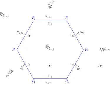
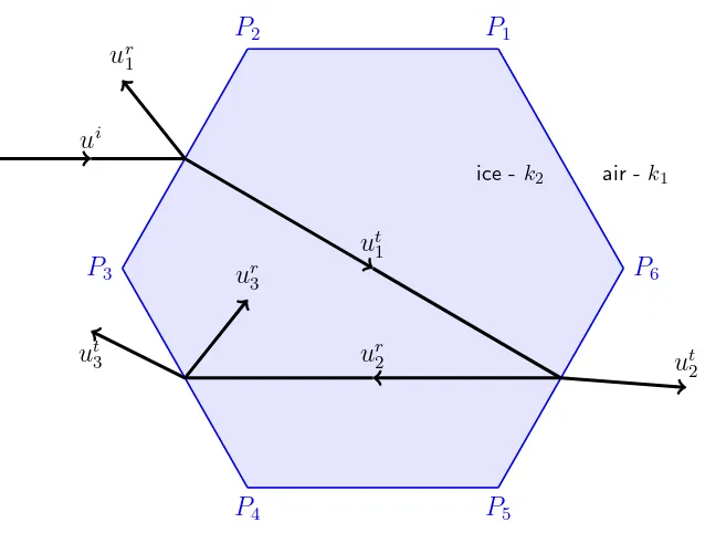
The notational setup can be seen in Figure 4.1. The notation is defined formally as follows. Let D denote the bounded open domain within the convex polygon and

Dc _:=_R2_\_D _{be the unbounded exterior domain. The boundary of} _D _{is Γ :=} _∪n i=1Γi,

where Γi, i = 1, . . . , n, are the n sides of the polygon. The incident plane wave ui

is directed from the top left of the figure towards the polygonal scatterer. Once this wave strikes Γ, it is partially reflected back into Dc _{and partially transmitted into} _D_.

The scattered field us _{comprises this initially reflected light as well as that which is}

transmitted into the shape, and then out again. We refer to the field inD by ut_{, so}

(29)

4.1. THE SETUP 21

whereut _{is the ‘transmitted’ field and denote the field outside the scatterer (in} _Dc_{) by}

u, so

u=us+ui, inDc_.

The scattered lightus and the transmitted lightut both satisfy the Helmholtz equa-tion, i.e.

(∆ +k1)us = 0 inDc, (4.1)

(∆ +k2)ut = 0 inD, (4.2)

wherek1 and k2 are the wavenumbers forus and utrespectively. Their ratio is equal to that of the refractive indicesm1 and m2, i.e.

k1 k2 =

m1 m2.

Equations (4.1)–(4.2) are supplemented by the boundary conditions

[u] = 0 on Γ, (4.3)

where n is the normal to Γ pointing into Dc_{. We also require for uniqueness that the}

scattered field us _{satisfies the} _{Sommerfeld radiation conditions}_,

us(x) = O r−1/2, (4.5)

∂us

∂r (x)−iku

s₍_x_{) =} _{o r}−1/2_, _(4.6)

as r _{→ ∞} where r = _|x_|, and the limit holds uniformly in all directions. In fact, we need only state the second condition since it can be shown that the first follows on from

the second. However, it is useful to consider both to assist the physical interpretation. The first condition means that_|u_|2 _{decreases in proportion to 1}_/r _as _r _{goes to infinity.}

Considered physically, this seems perfectly reasonable since as the light radiates out-ward from its source, the energy of the light (which is proportional to _|u_|2_{) is spread}

(30)

saying that far away from the scatterer the light wave appears locally like a plane wave

travelling in the direction of increasingr (i.e. outward from the source) [5].

Existence and uniqueness of the solution to the transmission problem can be proved under certain assumptions made on the wavenumbersk1 andk2, as detailed in [8], p.386.

We highlight one sufficient condition from [8] for existence and uniqueness which is of relevence to our particular setup, which is that we require

k1 >0 and k2 >0. (4.7)

Throughout we takek1 = 1 andk2 = 1.31, so we can be assured that our problem has a unique solution.

4.2 Integral Equation Formulation

In this section we employ the so called direct method as used by Silveira [17] (see also [7, _§3.2]) to derive an integral equation formulation which reduces the number of

dimensions of the problem from two to one. This is done using Green’s theorems. We state these for a bounded domainV with aC2 _{boundary and suppose that the functions}

φ, ψ _∈ C2(V)_∩C(V) have normal derivatives on the boundary ∂V in the sense that the limit

∂φ(x)

∂n = limh→0(n(x),∇φ(x−hn(x))), forx∈∂V, (4.8)

exists uniformly on ∂V, and a similar condition holds for the normal derivative of ψ. Then this suffices to ensure that Green’s first theorem

Z

are both valid. We have stated Green’s theorems for the case where V is a bounded

(31)

4.2. INTEGRAL EQUATION FORMULATION 23

polygonal domain is a Lipschitz domain. In this case we must state Green’s theorems

in a slightly different manner. We will not present this statement here but refer the reader to [14] for a rigorous exposition.

Firstly we note that the fundamental solutions of the Helmholtz equations (4.1)–

(4.2) are

whereH₀(1)(_·) is the Hankel function of the first kind of order zero (see [1] for properties

of this function). Now, applying Green’s second theorem (see Theorem 3.1 of [7] for details) to ut _{and Φ in} _D_{, we obtain}

Then applying Green’s first theorem as in Theorem 3.3 of [7] in Dc _{we arrive at}

Z

Combining (4.12) and (4.13) we obtain the integral representation for the transmission problem

so we may then add this term and ui _{to both sides of equation (4.15) to obtain an}

integral equation for the entire field u as opposed to merely the scattered field. This

(32)

Now we let x _→ Γ in equations (4.14) and (4.17) from D and Dc _{respectively, and}

utilising the jump conditions for layer potentials (see e.g. [5]), we obtain

u−₍_x_{) =}

and D respectively. Similarly, taking the normal derivatives to equations (4.14) and (4.17) in the limitx_→Γ from both sides shows that

∂u−₍_x₎

The equations (4.18)–(4.21) may be written in a more concise form by defining the

boundary integral operatorsSj, Kj,Kj′ and Tj for j = 1,2, as

(33)

4.2. INTEGRAL EQUATION FORMULATION 25

It follows from considering the boundary conditions (4.3) and (4.4) that only two of the unknown quantitiesu+_, _u−_, _∂u+_/∂n _and _∂u−_/∂n _{are linearly independent, in fact}

on the boundary Γ, u+ ₌ _u− ₌ _u _and _∂u−_/∂n ₌ _∂u+_/∂n ₌ _∂u/∂n_{. We resolve this}

issue by adding the first pair (4.26)+(4.27) and adding the second pair (4.28)+(4.29)

and combining them with the boundary conditions (4.3)–(4.4) to give the following system of coupled boundary integral equations (and dropping _± superscripts),

(I+K2₋K1)u+ (S1₋S2)∂u

These equations may be written in a matrix form as

(34)

We remark here that other formulations are possible by combining (4.26)–(4.29) in

different ways, see e.g. [12]. We can now solve the system (4.32) numerically foru and

∂u/∂n on the boundary Γ and then use equations (4.14) and (4.15) to calculate the

entire field inR2_{. One standard type of numerical method for solving the matrix system}

(4.32) is called the boundary element method.

4.3 Boundary Element Method

The boundary element method (BEM) can be seen as a finite element method (FEM)

applied to a problem that has been reformulated as a boundary integral equation. In this section we will consider only the simplest BEM (as detailed in [5]) in which the boundary

Γ is divided into M equally sized boundary elements, denoted by γ1, γ2, ..., γM. Along

each element we approximate the solution of the boundary integral equations (4.32) by

a polynomial of degree zero (i.e. a constant), souand∂u/∂nare approximated in each element γj by uj and vj, respectively, for j = 1,2, ...M. Since

We then use the collocation method to obtain a set of equations which determine the constantsuj and vj. The collocation method involves choosing so calledcollocation

(35)

4.3. BOUNDARY ELEMENT METHOD 27

(4.37) hold exactly at each of these points. We therefore require that, fork = 1, ..., M,

uk = ui(xk)−

This generates a linear system of 2M simultaneous equations to determine the 2M

(36)

if M + 1_≤k _≤2M. We can rewrite (4.40) as

AU=b, (4.42)

where

A:=I+B.

After assembling our matrix A, the next step is to solve the matrix system (4.42)

to obtain U. We may then use Green’s representation theorems (4.14) and (4.15) to calculate the field at any point in the domain.

The computational cost of this BEM scales with the size parameter X (which was defined in Chapter 1) since the mesh we use requires 10 elements per wavelength in

order to capture the wave behaviour accurately. Hence it is easy to see that for large

X the computational power required becomes too large for most machines. The output

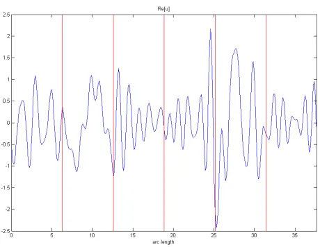
of using such a BEM can be seen in Figures 4.2(a) and 4.2(b). The BEM code used in this thesis is provided courtesy of David Hewett. Figure 4.2(a) shows the field u

on the boundary of the shape. Equations (4.14) and (4.15) tell us that knowledge of

u and ∂u

∂n on the boundary are sufficient to determine the field in R

2_{, which is shown}

in Figure 4.2(b). In Figure 4.2(b) the diffraction effects can be seen propagating into the shape from the 4 corners which are first hit by the incident light. It is these effects

(37)

4.3. BOUNDARY ELEMENT METHOD 29

(a) Real part ofu_{on boundary. The vertical red lines represent the}

corners of the hexagon, the first corner at 0 arc length is the one

located at the top-right of the hexagon. Arc length increases as we

go anti-clockwise around the boundary.

(b) Incident light with wavenumber k _{= 5 and amplitude} A _{= 1}

irradiates the hexagon from the top left. Plot shows the real part

ofu_{in the entire domain.}

Figure 4.2: Plots showing the approximation to the field produced by the boundary

(38)

Chapter 5 Ray Tracing Algorithm

In this chapter we apply the high frequency ray tracing method to obtain an approxi-mation to the field on the boundary of the polygon.

When the incident plane wave strikes the ice crystal, it will be diffracted and

re-flected. The new directions of these diffracted and reflected beams will depend upon which side of the polygon the light has hit. Since we consider a plane wave which

stretches to infinity in the directions perpendicular to its propagation, it will likely hit more than one side. In ray tracing we suppose each side which is ‘illuminated’ by the

incident light gives rise to two beams, one reflected and one transmitted, travelling in new directions. The task of a ray tracing algorithm is to follow the transmitted beams

as they travel around inside the shape and each time a beam strikes a side (see Fig-ure 1.2), the RTA calculates the new transmitted and reflected beams along with their

directions and amplitudes. The RTA then continues to track these new beams and so

on ad infinitum.

Of course, it is not possible to perform these calculations for infinitely many reflec-tions/transmissions so we must truncate the algorithm after a certain number of these

reflections, call this numberM. We may then evaluate the field on the boundary of the shape by summing the contributions from each of the beams. In Figure 5.1 the first

(39)

31

transmitted beam is denoted byut

1 and subsequent transmitted beams which leave the

shape are denoted ut

j, for j = 2, ..., M. Similarly, the first reflected beam is ur1, the

other reflected beams arise from the initial transmitted beam, these are written as ur j,

forj = 2, ..., M. Therefore the field on the boundary, approaching from the interior is

u=ut₁+

M

X

j=2

ur_j +ud, (5.1)

whereudis the field due to diffraction. Likewise, if we evaluate the field on the boundary,

approaching from the exterior we find

u=ui ₊_ur

These evaluations shall be elaborated upon in _§5.3.

In this chapter we derive the necessary equations for designing a RTA. These equa-tions include Snell’s Law and the Fresnel equaequa-tions, of which various derivaequa-tions are

(40)

32 CHAPTER 5. RAY TRACING ALGORITHM

to many, and in a coordinate invariant form, which will be convenient for

implementa-tion. We note that a published reference including similar derivations is not known to the author. Later in the chapter, in_§5.3, we discuss some of the results obtained from

implementing the RTA and pose questions which are to be resolved in the following chapter. But first, let us begin with one of the most fundamental laws of optics.

5.1 Snell’s Law

Snell’s Law describes the relationship between the angles of incidence and transmission when light waves pass from one isotropic medium into another, in our case we are

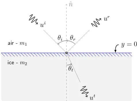
concerned with the two media air and ice. As can be seen in Figure 5.2 the angle of incidence θi is the angle measured anti-clockwise from the outward pointing normal ˆn

(directed out of the ice) to the direction vector of the incident light ui_{. Similarly the}

angle of transmissionθt is the angle measured anti-clockwise from the inward pointing

normal to the direction vector of the transmitted lightut_{. In addition to deriving Snell’s}

law, we also must state the law of reflection which we quote from [9]. Hence we must

also define the angle of reflectionθr; this is the angle measured anti-clockwise from the

direction vector of the reflected lightur _{to the outward pointing normal.}

To begin with we consider, for simplicity, a setup in which the boundary between ice and air passes through the origin of our general coordinates (x, y), more specifically

we take our boundary to bey= 0. We also utilise the boundary conditions (4.3)–(4.4) which we restate for convenience,

[u] = 0,

∂u ∂n

= 0, (5.3)

both ony = 0.

Now suppose a two-dimensional incident plane waveui _{with direction}_di _{strikes the}

(41)

5.1. SNELL’S LAW 33

ˆ

n

ui

θi

ut

θt

ur

θr

air -m1

ice -m2

y= 0

Figure 5.2: Refraction and reflection of light at the interface y= 0

transmitted with directiondt. The law of reflection [9] states that

θr =θi, (5.4)

and so we may write these direction vectors in the following form

di = (sinθi,−cosθi), dr = (sinθi,cosθi), dt= (sinθt,−cosθt). (5.5)

The general form of a plane wave is u = Aeikx_·d

where A is the amplitude, x the position,k the wavenumber anddthe direction vector of the wave. So, using (5.5), the

incident plane wave may be written as

ui =Aieik1(xsinθi−ysinθi)_, _(5.6) whereAi _{is the amplitude and the wave propagates in the half-plane} _{y >}_{0. The total}

field iny >0 in this scenario isu=ui₊_ur _where

ur=Areik1(xsinθi+ysinθi)_, _(5.7) is the reflected wave. In the half-plane y < 0 the total field is u = ut _{where the}

transmitted wave is

(42)

Herek1 and k2 represent the wavenumbers of the wave in air and ice respectively, and

are related by

k1 k2 =

m1 m2 =

c2

c1, (5.9)

where m1 and m2 are the refractive indices of air and ice as stated previously and c1

and c2 are the wavespeeds of light in these two media, respectively. The relationships

between the amplitudesAi_,_Ar _and _At _{will be derived later in} _§_{5.2 and}_§_5.2.1.

We now consider the the first of the boundary conditions (5.3); this implies that

ui₊_ur ₌_ut_. _(5.10)

Substituting for the u’s using (5.6)–(5.8) and noting that y = 0 on the boundary we have

Aieik1xsinθi₊_Ar_eik1xsinθi ₌_At_eik2xsinθt_, _(5.11)

and rearranging finally gives

Ai₊_Ar

At e

ix(k1sinθi−k2sinθt) _{= 1}_. _(5.12) Equation (5.12) must hold for all x_∈C_{, which implies}_{Snell’s Law of Refraction}

k1sinθi−k2sinθt= 0. (5.13)

This also implies that the amplitudes are related by

Ai+Ar=At. (5.14)

5.1.1 Snell’s Law in vector form

We have derived Snell’s Law for the case when the boundary aty = 0 as in Figure 5.2.

However, in our polygon in Figure 5.1 each side represents a boundary in a different position and orientation. In order to cope with a boundary in any position or orientation

(43)

5.1. SNELL’S LAW 35

upon the angles θi, θr and θt. This is because each time we are on a new boundary,

the normal to that boundary will be different from the normal to the previous one, which means that we must define a new way to measure these angles each time. In this

subsection we demonstrate how to find these new expressions.

The expressions in (5.5) show how the directions di, dr and dt can be written in terms of the incident and transmitted angles when we take the interface to be y = 0.

In this particular example, we may decompose the incident direction vector, say, into

x- andy- components respectively as

di = (sinθi,−cosθi)

For a general vector, d, we may do a similar operation but this time decompose com-ponents which are tangential and normal to the boundary,

d= d₋(d_·n)n

Using (5.15) and Snell’s Law (5.13), dt can be written as

dt = (sinθt,0) + (0,−cosθt)

Similarly, the expression for the reflected direction is found to be

(44)

5.2 Fresnel Equations

In section 5.1 we found one relationship between the 3 quantitiesAi_{, A}r _and_At_{, namely}

equation (5.14). The Fresnel equations provide two more relations between these am-plitudes which allow us to determine their values. Here we will derive the Fresnel

equations, firstly in the setup described in section 5.1, in which the interface between the two media is the line y= 0 (as in [10]), and secondly in a more general setup.

Writing the second of the boundary conditions (5.3) using the plane wave form

u=Aeikx_·d

and using (5.10), we have

−ik1cosθiui+ ik1cosθiur =−ik2cosθt(ui+ur),

which after cancellation and rearrangement becomes

ur = k1cosθi−k2cosθt

k1cosθi+k2cosθt

ui. (5.18)

Now, on y = 0, ur ₌ _Ar_eik1xsinθi and ui = Aieik1xsinθi so from (5.18) we obtain an

expression for the reflection coefficient which is the first of the Fresnel equations,

R := A

is the relative refractive index. Notice that when 1/ζ >1 (which is the case when the light travels from the air into the ice, in fact here 1/ζ = 1.31) andθi <arcsin(1/ζ),α is

real and positive. This implies that_|R_|<1 and so the amplitude of the reflected wave is smaller that the amplitude of the incident wave. Also, by Snell’s Law (5.13),θt < θi,

so the effect of refraction is to ‘bend’ the light towards the normal to the boundary, a physical phenomenon which was explained in _§3.3 using a more intuitive (but less

(45)

5.2. FRESNEL EQUATIONS 37

However, when 1/ζ < 1 (i.e. when the light travels back out of the ice crystal into the

air, here 1/ζ = 0.76) it is possible for α to be imaginary. In fact, α is imaginary when the incident angle θi exceeds the critical angle θc = arcsin(1/ζ). In this case |R| = 1

and the amplitude of the transmitted wave is equal to that of the incident wave. There is still a transmitted wave, however it is exponentially decaying asy _{→ −∞}[10]. This

phenomenon is known astotal internal reflection. This name is useful as it tells us that it only occurs on the interior of the ice crystal.

Now we derive the second of the Fresnel equations. From (5.14) we know that

1 + A

where T := At_/Ai _{is the transmission coefficient. Hence the second of the Fresnel}

equations is

T = 2 cosθi cosθi+α(θi)

. (5.24)

It can easily be shown that the vector form of the Fresnel equations is

R = d

The Fresnel equations stated in the previous section were derived under the assumption

that one of the coordinate axes coincides with the interface. When tracking light beams around the interior of the polygon and considering the interaction of the beams with

(46)

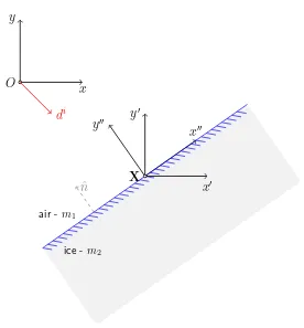
in terms of a single coordinate system but relevant for interfaces that lie away from the

origin of this system and are not aligned with these coordinate directions as illustrated in Figure 5.3.

y′′

x′′

ˆ

n

air -m1

ice -m2

y′

x′ y

x O

di

X

Figure 5.3: Coordinate shift and rotation.

Suppose X is a point on the interface and O is the origin of the general coordinate

system. The coordinate system (x, y) is our general system and the coordinates (x′′_{, y}′′₎

are equivalent to those used in Figure 5.2 since they are in the plane of the interface.

To transform from (x, y)– to (x′_{, y}′_{)–coordinates we simply shift by}_X_,

x′ =x₋X. (5.28)

Then in order to transform from (x′_{, y}′_{)– to (}_x′′_{, y}′′_{)–coordinates we rotate using a}

rotation matrixM,

(47)

5.2. FRESNEL EQUATIONS 39

whereM is orthogonal, i.e. it satisfies MTM =M MT = 1. So, combining (5.28) and

(5.29) we obtain

x′′ =M(x₋X), (5.30)

which is the transformation from (x, y)- to (x′′_{, y}′′_{)-coordinates.}

Let us begin by rewriting the representations of the incident, reflected and

trans-mitted rays (5.6)–(5.8) in vector form as

ui = Aiexpik1di_·x , (5.31)

ur = Arexp_{ik1dr_·x_}, (5.32)

ut = Atexpik2dt_·x . (5.33)

In order to derive the desired Fresnel equations we must transform (5.31)–(5.33) into (x′′_{, y}′′_{)-coordinates, solve the problem as in} _§_{5.2, then transform back into general}

coordinates. In (x′′_{, y}′′_{)-coordinates we have}

ui = Ai′′expik1(di)′′_·x′′ , (5.34)

ur = (Ar)′′exp_{ik1(dr)′′_·x′′_}, (5.35)

ut = At′′expik2(dt)′′_·x′′ , (5.36)

where x′′ =M(x₋X), (di)′′ ₌_M−1_di _{and (}_Ai₎′′ _{etc. are to be determined. Starting}

with (5.34) and expanding gives

ui = Ai′′expik1 M−1di_·(M(x₋X)) = Ai′′expik1di_·(x₋X)

= Ai′′exp₋ik1di_·X expik1di_·x . (5.37) Similarly for the reflected and transmitted waves we have

ur = (Ar)′′exp_{−ik1dr_·X_}exp_{ik1dr_·x_} (5.38) and

(48)

By comparing (5.37)–(5.39) with (5.31)–(5.33) we notice that

Ai ₌ _Ai′′_exp₋_i_k

The reflection coefficientR in general coordinates is defined as the ratio of the reflected amplitude to the incident amplitude, so we may now write

R:= A

whereR′′ _{is the reflection coefficient on the boundary} _y′′ _{= 0 which is calculated as in}

(5.25). The term multiplyingR′′ _{in (5.44) represents a phase shift due to the offsetting}

of the origin from the interface. Using the same method but for T′′ _{:= (}_At₎′′_/₍_Ai₎′′

Note the sgn(di_·n) which has been included so that the expression is valid on the interior of the shape also, since here the normal directions to the sides are reversed.

It is important to note that the equations derived in this chapter are valid for the scenario when light is propagating into the ice crystal, i.e. from air to ice. In order to

make them valid for the scenario when light is propagating out of the ice crystal, all we need to do is switch the refractive indices k1 and k2. This is easily implemented

in the algorithm since the first scenario mentioned is relevant only for the inital wave transmission/reflection, that is when ui _{his the crystal and splits into} _ur

1 and ut1 in

(49)

5.3. EVALUATING THE BOUNDARY DATA 41

5.3 Evaluating the boundary data

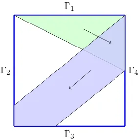
As an example, we consider a square crystal illuminated from the top left, as in Fig-ure 5.5. The incident plane wave will strike sides Γ1 and Γ2 of the crystal, giving rise

to a transmitted and reflected beam from each. Figure 5.4 shows the transmitted beam from Γ1 and the reflected beam it causes once it strikes Γ4, this beam will strike sides

Γ2 and Γ3 giving rise to more beams and so on. The formulae derived in §5.1 and §5.2

govern the directions of these reflected and transmitted beams, and the amplitudes of

their associated fields. So once these formulae are programmed in the form of a RTA code and run on a computer for M reflections/transmissions, we will build up a large

array of data which gives us the details of: the number of beams which have hit each side, their widths and positions, and their transmitted and reflected directions and

amplitudes.

Γ1

Γ2

Γ3

Γ4

Figure 5.4: Ray tracing inside the polygon. Note that the transmitted rays have not been included in this diagram.

In order to evaluate the contribution to the electric field of each of these beams, we

use the formula

u(x) = Aeikd_·x

. (5.46)

(50)

beams bouncing around inside the crystal, and also an array of beams transmitted out

of the crystal, so which do we choose when evaluating the field? Due to the boundary condition [u] = 0, either may be chosen so long as we remain consistent.

So, (using the notation from Figure 5.1) summing the beams in the interior leads to

the ray tracing approximation for the boundary field (or leading order behaviourul) as

ul =ut1 +

M

X

j=2

ur_j. (5.47)

Whereas if we sum the beams which are propagate away from the shape, we have

ul =ui+ur1+

j and urj are calculated using the formulae (5.35)–(5.36) derived in §5.2.1. We

choose the first option (5.47) in our implementation. Note that (5.47)–(5.48) differ from

(5.1)–(5.2) in that the first two do not includeud. This is because (5.47) and (5.48) are

the fields given by the RTA, which does not account for diffraction, so the fields will

have noud term.

Now let us look at some outputs from our implementation of the RTA. Consider the setup illustrated in Figure 5.5 in which a square ice crystal with refractive index

m2 = 1.31 is irradiated from the top left by a plane wave with wavenumber k = 5 and amplitudeA = 1. The length of each side is 2π so that 5 wavelengths of light fit along

each side, this also ensures that the size parameter X is equal to k. The origin of the coordinate system is located at the centre of the square. Figure 5.6 shows the real and

imaginary parts of u around the boundary for M = 50. The vertical red lines depict the corners of the square going anti-clockwise from θ = 0, which we choose as P1. So

the first red line represents P2, the second P3, etc. Note that the field on the first two sides, Γ1 and Γ2, are symmetrical, as are the fields on the final two, Γ3 and Γ4. This is

a consequence of the origin’s location at the centre of the shape and the 45◦ _incident

angle of the light. If we were to shift the origin or alter the incident light’s direction,

(51)

P2 Γ1

P3

Γ2

P4

Γ3

P1

Γ4 y

x O ui

Figure 5.5: Setup for the square with P1 = (π, π), P2 = (₋π, π), P3 = (₋π,₋π) and

P4 = (π,₋π).

suggests that more light is transmitted through the shape than is reflected away from

the illuminated sides Γ1 and Γ2. This is intuitive because we know from experience that

ice is transparent. If we were to make the refractive index of the scatterer very large,

the reverse would be true. Increasing the refractive index is equivalent to making the scatterer more opaque.

Figure 5.7 shows how the field changes after each reflection/transmission. The first plot shows the field on the boundary after only Γ1 and Γ2 have been illuminated by the

incident light. The second plot shows the field after the light has passed into the top left of the square and out of the bottom right, which at first thought might seem to be

enough tracking of the ray as to give a good representation of the field. However from looking at the later plots, it is evident that the contributions from subsequent internal

reflections have a significant effect on the total field on the boundary (although the contributions diminish with each reflection as we shall see in the next chapter).

An interesting question arises here: How many internal reflections, M, is it

(52)

Figure 5.6: Ray tracing approximation withM = 50 of the electric field on the boundary of the square ice crystal in Figure 5.5 which is being irradiated by light with wavenumber

k= 5, amplitude A= 1 and direction di = (1,₋1).

If we can determine this, then we may use the answer to truncate the number of reflec-tions the algorithm calculates, hence saving on computing time. Other quesreflec-tions stem

from this, such as How does M depend on the wavenumber, the amplitude or the shape

of the obstacle?.

Once we ascertain M, we may make fair comparisons between the fields generated

by the RTA and BEM. Recall that the RTA does not incorporate diffraction, whereas the BEM does. So by comparing the outputs of these two methods we may be able

to isolate the effects of diffraction. Questions we hope to answer are What form do

diffraction effects take? and Is there a precise formula that captures the behaviour of

(53)

Figure 5.7: Ray tracing approximation of the electric field on the boundary of the square crystal in Figure 5.5 which is being irradiated by light with wavenumberk = 5,

amplitudeA= 1 and directiondi = (1,₋1). Each subsequent plot shows the field after considering one more reflection/transmission, so we go fromM = 1 to M = 4.

(54)

Chapter 6 Results and Discussion

This chapter discusses the questions posed at the conclusion of the previous chapter, in an attempt to better understand the behaviour of diffraction (the term ud) in our

problem. We first wish to ascertain how many reflections/transmissions (M) to consider in the RTA to obtain an accurate description of the leading order component of the

scattered field. This issue is dealt with in _§6.1.

Once the answer to this question has been established we may proceed to_§6.2 where we subtract the leading order behaviour obtained by ray tracing, from the

approxima-tion obtained using the BEM, in order to establish the importance, and study the influence, of diffraction.

6.1 Convergence of solution

This section discusses the questionHow many internal reflections, M, is it necessary to

track in order to obtain an accurate representation of the field on the boundary? Which is another way of asking: How quickly does the ray tracing approximation converge?

In order to analyse this convergence, we will take the field on the boundary after

(55)

6.1. CONVERGENCE OF SOLUTION 47

50 reflections (M = 50) as the ‘exact’ solution1_, _U_{, and will evaluate the Euclidean or}

l2_{-norm of the difference between the exact solution and the solution after}_M _reflections

forM = 1,2, ...,49, i.e.

whereL is the number of grid points around the boundary at which u is calculated.

Figure 6.1(a) shows a logarithmic plot of errorM against M for the scenario in

Figure 5.5 with varying k. Straight lines on a log plot imply that the convergence

to the exact solution is exponential, in fact, for the square the equation of the line is roughly

It is of note that the figure suggests that β is independent of k. Also it is worth

mentioning that the slight divergence of the lines after M = 40 can be ignored since at this point the error is 10−16 _{which is machine precision, so we may assume that the}

data after this point is unreliable. This would imply that, in order to obtain machine precision with the RTA, we may take M = 40 as sufficient.

We remark that this rate of convergence is specific to the relative refractive index of ice to air, i.e. 1.31. If we increase the refractive index of ice, to 2 for example, we

can expect a much slower convergence as is verified by Figure 6.2. We see here that the RTA requires M = 60 to reach machine precision. This is because for a higher

refractive index, the incidence of total internal reflection is more common. Why total internal reflection is important to the convergence of the ray tracing algorithm shall be

studied in the following subsection.

1

In this section we use the word ‘solution’ to refer to the ray tracing approximation, and the phrase

(56)

48 CHAPTER 6. RESULTS AND DISCUSSION

6.1.1 Exponential convergence and geometric series

The exponential convergence of the ray tracing method to the exact solution can be explained by comparing the series of reflected beams to a geometric series. As the

bundle of light beams are reflected around inside the shape, the amplitude of each reflected beam is smaller than its preceeding one by a factor of R (where R is the

reflection coefficient) unless total internal reflection occurs. A series in which successive terms share a common ratio is ageometric series, i.e. a series of the form

a+ar+ar2+ar3+..., (6.3)

wherer is the common ratio.

For a ray travelling around inside the square of ice with incident light directed at

45◦ to the illuminated sides (as in Figure 5.5), the ray will undergo either total internal reflection or reflection with coefficientR= 0.2186. If we ignore total internal reflection

and phase shift, the geometric series for the amplitude of this ray is

A+AR+AR2+...+ARM−1 =A1−R

M

1₋R , (6.4)

whereAis the amplitude of the incident light. The sum of the infinite series isA/(1₋R), so the error incurred by truncating afterM reflections is

A

Plotting this alongside the RT error decay (see Figure 6.3) shows us that the con-vergence of the geometric series is faster. But this is probably due to ignoring total

internal reflection in which_|R_|= 1. Although the convergence plots do not match, the qualitative comparison is instructive.

Indeed, formula (6.5) suggests that the rate of convergence is dependent onR, so ifR

is usually small, then the solution should converge quickly and if it is usually large, the solution should converge more slowly. This equates to saying that the obstacle shape

(57)

6.2. RAY TRACING VS. BEM 49

We might expect that shapes with more sides will cause a slower rate of convergence

since the angles of incidence (recall this angle is measured from the normal to each side as in Figure 5.2) within the shape are more likely to be large, and hence there is a

greater chance of total internal reflection and R in general will be large. Figure 6.1(b) demonstrates how this rate varies for different shapes. Note that the regularly spaced

kinks are due to total internal reflection.

Although we have seen that (6.5) is not a true representation of errorM, it can be

seen as a lower bound on this error. Also it can be used to determine roughly how much

faster or slower one particular setup will converge compared to another. By setup, it is meant the combination of incident light angle and obstacle shape. For example, one

need only perform a few calculations ‘by hand’ using the Fresnel formula (5.19) for the two setups to find a common or ‘characterstic’ value ofR for each, input this value into

(6.5) and compare the results.

Formula (6.5) also suggests that the rate of convergence should be independent of

the wavenumber, which is consistent with the results shown in Figure 6.1(a). This result demonstrates that ray tracing is a frequency independent method and so is considerably

more efficient than the BEM for high frequencies.

6.2 Ray Tracing vs. BEM

The main objective of this thesis is to examine the difference, ud, between the exact

solution2 _u _{and the leading order behaviour} _u

l and in this section we do exactly this.

The BEM takes into account the diffraction of light from the corners of the obstacle, which is a physical feature that is not picked up using our ray tracing technique. So

we expect some difference between the two solutions. Figure 6.4(a) shows ucalculated using the two different methods. The setup is again as shown in Figure 5.5, i.e. a square

2

In this section we return to the original use of the term ‘solution’, i.e. the exact solution refers to

(58)

50 CHAPTER 6. RESULTS AND DISCUSSION

crystal being illuminated from the top left. The angle θ in Figure 6.4(a) is measured

in radians anti-clockwise from the first corner P1, at which θ= 0. The corner which is first hit by the incident light is P2 which is located at θ =π rad in Figure 6.4(a) (also

shown by the first vertical red line from the left). We notice good agreement on the illuminated sides Γ1 and Γ2 between the two approximations as well as at P4, however

along the shadow sides, Γ3 and Γ4, the agreement is considerably weaker which suggests

that the diffraction effects are large on the sides in shadow as well as on the shadow

side of cornersP1 and P3.

Figure 6.4(b) showsudalone. This plot better identifies the regions which have been

affected most by the effects of diffraction from the corners of the square. The regions

of large ud are on sides Γ3 and Γ4 which is to be expected since the diffracted light

is propagating from the corners in the top left through the shape towards the bottom

right. For this particular scenario, with k = 10, ud is fairly uniform over these two

sides, this is because diffraction effects are large for a low wavenumber such as this,

so they will spread out over a wide region. It would be instructive to look to higher frequencies, where the diffracted regions are narrower, in order to seek a pattern. But

how do we know which frequencies are good to use for this purpose? In order to answer this, we choose some measure of the difference between the two approximated fields and

analyse its behaviour as k increases. We do this in the next subsection and return in

§6.2.2, better informed, to the task of ascertaining the effect of diffraction on the field around the boundary.

6.2.1 Relative Error

As the frequency of the incident light is increased, the effects of diffraction diminish

and so we expect the outputs from the BEM and RT to become more similar. By considering the relative error between the two solutions it is possible to see precisely

Light scattering by penetrable convex polygons

University of Reading

School of Mathematical and Physical Sciences