Chapters of This Lesson

(1)

ALGORITMA PEMROGRAMAN 2

PROCESSING

(2)

Chapter 1 :

Pixels

Chapter 1 :

Pixels

Chapter 2 :

Processing

Chapter 2 :

Processing

Chapter 3 :

Interaction

(3)

Chapter 1 :

Pixels

(4)

Chapters of Pixels

1.

In this chapter :

 Specifying pixel coordinates

 Basic shapes: point, line, rectangle,

ellipse.

 Color: grayscale, “RGB”

(5)

1.1 Graph Paper

 The shortest distance between two points

(6)

1.1 Graph Paper

 The instruction will look like this for Figure

1.1 :

 This is the frst line of computer code in

Processing.

(7)

1.1 Graph Paper

 In addition, we are specifying some

arguments for how that line should be drawn, from point A(0,1) to point B(4,5).

 The code sentence also end with a

(8)

1.1 Graph Paper

 The key here is to realize that the

compiter screen is nothing more than a

fancier piece of graph paper.

 Each pixel of the screen is a coordinate –

two numbers, an “x” (horizontal) and a “y” (vertical) that determine the location of a point in space.

 And it is our job to specify what shapes

(9)

1.1 Graph Paper

 The graph paper from eight grade

(10)

1.1 Graph Paper

 The coordinate

system for pixels in a computer window, however, is reversed along the

y-axis (0,0) can be found at the top left with the positive direction to the right direction

(11)

1.2 Simple Shapes

 The students you may ultimated learn to

develop interactive games, algorithmic art pieces, animated logo designs, and (insert your own category here) with

Processing, but at its core, each visual program will involve setting pixels.

 The simplest way to get started in

(12)

1.2 Simple Shapes

 The Four Primitive Shapes in Figure

(13)

1.2 Simple Shapes

 In each of the diagrams in Figure 1.5,

(14)

1.2 Simple Shapes

 A point is the easiest of the shapes and a

good place to start.

 To draw a point, we only need an x and y

(15)

(16)

1.2 Simple Shapes

 Once we arrive drawing a rectangle, things

become a bit more complicated.

 In Processing a rectangle specifed by the

(17)

(18)

1.2 Simple Shapes

 From Figure 1.7 indicate that the default

mode is “CORNER”, which is how began as illustrated in Figure 1.7. We Prefer this method, we frst indicate that we want to use the “CENTER” mode before the instruction for the rectangle itself.

(19)

(20)

(21)

1.2 Simple Shapes

 Once we have become comfortable with

the concept of drawing a rectangle, an ellipse is a snap.

 In fact, it is identical to rect() with the

diference being that an ellipse is drawn where the bounding box (as shown in Figure1.11) of the rectangle would be.

 The default mode for ellipse() is

(22)

(23)

(24)

(25)

1.2 Simple Shapes

 It is important to acknowledge that in Figure 1.10, th

ellipse do not look particularly circular.

 Processing has a built-in methodology for selecting

which pixels should be used to create a circular shape.

 Zoomed in like this, we get a bunch of squares in a

circle-like pattern, but zoomed out on a computer screen, we get a nice round ellipse.

 Later, we will see that Processing gives us the power

(26)

(27)

(28)

1.2 Simple Shapes

 Triangle()

 Arc()

 Quad()

(29)

1.2 Simple Shapes

 Exercise 1-2: Using the blank graph

(30)

1.2 Simple Shapes

 Exercise 1-3 : Reverse engineer a list

(31)

1.3 Grayscale Color

 In the digital world, precision is required.

Therefore, color is defned with a range of numbers.

 Let’s start with simplest case: black and

white or grayscale.

 In grayscale terms, we have the following:

(32)

(33)

1.3 Grayscale Color

 In Processing, every shape has a stroke()

or fll () or both.

 The stroke() is the outline of the shape,

and the fll() is the interior of tha shape.

 Lines and point can only have stroke(), for

(34)

(35)

1.3 Grayscale Color

 Note :

 If we forget to specify a color, Processing

will use black (0) for the stroke () and white (255) for the fll() by default.

 Assuming that before slide larger

(36)

1.3 Grayscale Color

 By adding the stroke() and fll() functions

before the shape is drawnn, we can set the color.

(37)

1.3 Grayscale Color

(38)

1.3 Grayscale Color

 Stroke () or fll() can be eliminated

(39)

1.3 Grayscale Color

(40)

1.3 Grayscale Color

 If we draw two shapes at one time,

Processing will always use the most recently specifed stroke() and fll(),

(41)

1.3 Grayscale Color

 Exercise 1-4: Try to guess what the

(42)

1.4 RGB Color

 Digital colors are also constructed by

mixing three primary colors, but it works diferently from paint.

 First, the primaries are diferent: red,

(43)

1.4 RGB Color

(44)

1.4 RGB Color

(45)

1.4 RGB Color

 Processing also has a color selector to aid

(46)

1.4 RGB Color

 Processing also has a color selector to aid

(47)

1.4 RGB Color

 Exercise 1-5 : Complete the following

(48)

1.5 RGB Color

 In addition to the red, green, and blue components of

each color, there is an additional optional fourth component, refered to as the color’s “alpha”.

 Alpha means tranparency and is particulary useful

when you want to draw elements that appear partially see-through on top of one another.

 The alpha values for in image are sometimes refered

to collectively as the “alpha channel” of an image.

(49)

1.5 RGB Color

 Behind the scenes, Processing takes the

color numbers and adds a percentage of one to a percentage of another, creating the optical perception of blending.

 Alpha values also range from 0 to 255, with

0 being completely transparent (i, e. 0% opaque) and 255 completely opaque (i,e., 100% opaque).

 Example 1-4 shows a code example that is

(50)

(51)

1.5 RGB Color

(52)

1.6 Custom Color Ranges

 RGB color with ranges of 0 to 255 is not the

only way you can handle color in Processing.

 Behind the scenes in the computer’s memory, color is always talked about as a series of 24 bits (or 32 in the case of colors with an alpha).

 However processing will let us think about color any way we like, and translate our values into numbers the computer understands.

(53)

1.6 Custom Color Ranges

 Specifying a custome mode with

colorMode().

 Although it is rarely convenient to do

(54)

1.6 Custom Color Ranges

 Now we are seting “Red values go from 0

(55)

(56)

(57)

Chapter 2 :

Processing

(58)

Processing

1. In this Chapter

 Downloading and installing Processing

 Menu Options

 A Processing sketchbook

 Writing Code

 Errors

 The Processing Reference

 The “Play” Button

 Your frst sketch

(59)

2.1 Processing to the

Rescue

2.1 Processing to the

Rescue

1.

The environtment we are going to use

is

Processing, free

and open source

software developed by

Ben Fry

and

(60)

Rescue

1.

Processing’s core

library of functions

for drawing graphics to what the code is

doing.

(61)

Rescue

1.

It is not some pretend language to help

(62)

2.2 How do I get

Processing?

2.2 How do I get

Processing?

1.

Processing

is

available

for

free

download.

2.

Head to

http://www.processing.org/

and visit the download page.

3.

If you are a Windows user, you will see

two option

“Windows (standard)”

(63)

2.3 The Processing

Application

2.3 The Processing

Application

1. The Processing development environtment is a simplifed environtment for writing computer code, and is just about as straightforward to use as simple text editing software (such as TextEdit or Notepad) combined with a media player.

(64)

2.3 The Processing

Application

(65)

2.3 The Processing

Application

(66)

2.3 The Processing

Application

2.3 The Processing

Application

1.

To make sure everything is working, it

iis a good idea to try running one of the

Processing examples.

2.

Go to FILE -> EXAMPLES -> Pick an

(67)

2.3 The Processing

Application

(68)

2.4 Coding in Processing

1.

There are

three of statements

we

can write:

 Function Calls

 Assignment Operations

(69)

1.

Every line of code will be a function call.

2.

We used functions to describe how to

draw shapes (we just called them

“commands” or “instructions”)

3.

Eah function call must always end with

(70)

1.

We have learned several functions

already, including :

 background(), rect()

 stroke(), ellipse()

 fll(), rectMode(),

 noFill(), ellipseMode().

 noStroke(),

 point(),

(71)

1.

Size() : function specifes the dimensions

of the window you want to create and

takes two arguments,

width

and

height

.

2.

The

size()

function should always be

frst.

(72)

(73)

(74)

(75)

1.

Example 2-4:

Create a blank sketch.

Take your code from the end of Chapter

1 and type it in the Processing window.

Add comments to describe what the

code is doing. Add

a println()

(76)

2.5 Erros

1.

In Figure 2.6 shows what happens when

you have a typo –

“elipse”

instead of

“ellipse” on line 9.

2.

If there is an error in the code

when

the play button is pressed

, Processing

will not open the sketch window, and will

instead display the error message.

(77)

2.5 Erros

(78)

2.5 Erros

(79)

2.5 Erros

1.

Exercise 2:6 :

Fix the errors in the

(80)

2.6 The Processing

Reference

2.6 The Processing

Reference

1.

The reference for

Processing

can be

found online at the ofcial web site (

http://www.processing.org

) under the

“reference” link.

2.

There, you can browse all of the

(81)

2.6 The Processing

Reference

(82)

2.7 Your First Sketch

1.

The example will follow the story of our

new friend Zoog, beginning with a static

rendering with simple shapes.

2.

Zoog’s development will include mouse

(83)

(84)

(85)

2.8 Publishing Your Program

1.

After you have completed a Processing

sketch, you can publish it to the web as

Java Applet.

2.

This will become more exciting once we

(86)

1.

Omce you have fnished Exercise 2-9

and determined that your sketch works,

(87)

(88)

(89)

2.8 Publishing Your Program

(90)

1.

Export to Windows 32

(91)

(92)

Chapter 3 :

Interaction

(93)

Interaction

1.

In This chapter:

 The “fow” of the program

 The meaning behind setup() and draw()

 Mouse Interaction

 Your frst “dynamic” Processing

program

 Handling events, such as mouse clicks and

(94)

3.1 Go with the fow



Focus on this chapter is that very “fow”

over time.



A game begins with a set of initial

conditions: you name your character,

you start with a score of zero, and you

start on level one. Let’s think of this

part as the program’s

SETUP.



After these conditions are initialized,

(95)

3.1 Go with the fow



This cycle of calculating and drawing

happens over and over again, ideally 30

or more times per second for a smooth

animation.



Let’s think of this part as the program’s

(96)

3.1 Go with the fow



This concept is crucial to our ability to

move beyond static design (as in

Chapter 2) with Processing.

 Step 1. Set starting conditions for the

program one time.

 Step 2. Do something over and over and

(97)

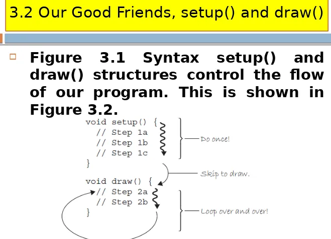
3.2 Our Good Friends, setup() and draw()



This chapter take this newfound

knowledge and apply it to our frst

“dynamic” Processing sketch.



Unlike Chapter 2’s static

examples,

this program will draw to the screen

continously (i.e., until the user quits).



This is accomplihsed by writing two

blocks of code

setup()

and

draw()

.

(98)

(99)

(100)

3.2 Our Good Friends, setup() and draw()

(101)

(102)

(103)

(104)

(105)

(106)

3.3 Variation with the Mouse



Consider this, what if, instead of typing

a number into one of the drawing

functions,

you

could

type

“

the

mouse’s X location” or “the

mouse’s Y location”

.

(107)

(108)

3.3 Variation with the Mouse

(109)

(110)

(111)

(112)



Just ,

move

background()

to

setup()

(113)



We could

push this idea a bit further

and create an example where a more

complex pattern (multiple shapes and

color) is controlled by

MouseX

and

MouseY

position.



For Example

, we can rewrite Zoog to

(114)



Note :



Zoog’s body is located at the exact

location of the mouse (

MouseX,

MouseY)

, however, other parts of

Zoog’s body are drawn relative to the

mouse.



Zoog’s head, for example, is located at

(115)

(116)

(117)

(118)

(119)

(120)

(121)



In addition to

mouseX and mouseY

,

you can also use

pmouseX

and

pmouseY

.



These two keywords stand for the

“previous”

mouseX

and

mouseY

locations, that is, where the mouse was

the last time we cycled through

draw()

.



For example, let’s consider what

(122)

(123)

(124)

3.4 Mouse Clicks and Key Presses



We know

setup()

happens once and

draw()

loops forever.



When does a mouse click occur? Mouse

presses

(and

key

presses)

as

considered

events

in Processing.



If we want something to happen (such

(125)



These are two new functions we need:



mousePressed()

–

Handles mouse

clicks.

(126)



Example 3-5:

mousePressed() and

keyPressed()



Adding squeres whenever the mouse is

(127)

3.4 Mouse Clicks and Key Presses



Example 3-5:

mousePressed() and

(128)



Example 3-5:

mousePressed() and

(129)

(130)

(131)

(132)

(133)

3.4 Mouse Clicks and Key Presses

(134)

(135)

(136)

(137)

Lesson One Project



(You may have completed much of this

project already via the exercises in

Chapters 1–3.



This project brings all of the elements

(138)

Lesson One Project



Step 1. Design a static screen

drawing using RGB color and

primitive shapes.

(139)

The End and Thank You



Shifman, Daniel. 2008.

Learning