A General Method for the Numerical Computation
of Manipulator Singularity Sets
Oriol Bohigas, Dimiter Zlatanov, Llu´ıs Ros, Montserrat Manubens, and Josep M. Porta
Abstract—The analysis of singularities is central to the devel-opment and control of a manipulator. However, existing methods for singularity set computation still concentrate on specific classes of manipulators. The absence of general methods able to perform such computation on a large class of manipulators is problematic because it hinders the analysis of unconventional manipulators and the development of new robot topologies. The purpose of this paper is to provide such a method for nonredundant mechanisms with algebraic lower pairs and designated input and output speeds. We formulate systems of equations that describe the whole singularity set and each one of the singularity types independently, and show how to compute the configurations in each type using a numerical technique based on linear relaxations. The method can be used to analyze manipulators with arbitrary geometry, and it isolates the singularities with the desired accuracy. We illustrate the formula-tion of the condiformula-tions and their numerical soluformula-tion with examples, and use 3-D projections to visualize the complex partitions of the configuration space induced by the singularities.
Index Terms—Branch-and-prune method, linear relaxation, nonredundant manipulator, singularity set computation.
I. INTRODUCTION
I
N robot singularities, either the forward or the inverse instan-taneous kinematic problem becomes indeterminate, and the properties of the mechanism change dramatically, often detri-mentally. Despite the importance of such critical configurations, the rich literature on singularity analysis does not provide a method to explicitly compute the singularity set, and to identify the various singularity types in it, on manipulators of a gen-eral architecture. Most works on the topic focus on particular classes of singularities and restrict their attention to specific robot designs [1]–[13].The efforts on characterizing all possible singularity types date back to the nineties [14]–[19]. Based on an input–output velocity equation, a general singularity classification was at-tempted in [14], but it was soon seen that this classification
Manuscript received May 6, 2013; accepted September 20, 2013. Date of publication October 18, 2013; date of current version April 1, 2014. This paper was recommended for publication by Associate Editor V. Krovi and Editor B. J. Nelson upon evaluation of the reviewers’ comments. This work was supported in part by the Spanish Ministry of Economy and Competitiveness under Contract DPI2010-18449. The work of M. Manubens was supported by a Juan de la Cierva contract.
O. Bohigas, L. Ros, M. Manubens, and J. M. Porta are with the Kinematics and Robot Design Group, Institut de Rob`otica i Inform`atica Industrial, CSIC-UPC, 08028 Barcelona, Spain (e-mail: [email protected]; [email protected]; [email protected]; [email protected]).
D. Zlatanov is with the PMAR Laboratory (DIMEC), Universit`a di Genova, 16145 Genoa, Italy (e-mail: [email protected]).
Color versions of one or more of the figures in this paper are available online at http://ieeexplore.ieee.org.
Digital Object Identifier 10.1109/TRO.2013.2283416
overlooks cases where the motion of the mechanism cannot be described solely with the input and output speeds [15]. This led Zlatanov to define a general manipulator model in terms of dif-ferentiable mappings between manifolds, giving rise to a rigor-ous mathematical definition of kinematic singularity [16], [18]. Using the model, six different singularity types were identified, which correspond to the distinct kinematic phenomena that may occur in a singularity.
Although the conditions for the presence of singularities of all types were given in [17] and [18], the formulation of these conditions into a form amenable for computation had yet to be achieved. The goal of the present work is to address this task by defining systems of equations that describe all singularity types and proposing a numerical procedure able to solve them. The methodology is general and applicable to virtually any relevant mechanism geometry. It allows the complete singularity set to be obtained with the desired accuracy and each of its singularity types to be computed independently.
The approach was preliminarily introduced in [20] and is now presented and illustrated in thorough detail. The guiding principle is the importance of a complete characterization of the manipulator motion in order to identifyallpossible singu-lar phenomena. For each such phenomenon, we present, simply and rigorously, the definition, the mechanical significance, the algebraic conditions, and the computation of the correspond-ing scorrespond-ingularity subset. Special emphasis is placed on illustratcorrespond-ing concepts and procedures with clear and comprehensible ex-amples. In addition, since a full knowledge of a mechanism’s special configurations is key to understanding its motion ca-pabilities, the paper exemplifies the use of 3-D projections to reveal and visualize the complex singularity-induced partition and interconnectedness of the configuration space.
The rest of the paper is organized as follows. Section II briefly recalls the definition of singular configuration and provides sys-tems of equations that characterize the whole singularity set of a manipulator. These systems can already be used to isolate the set, as done in [21] for the planar case; however, additional systems are provided in Section III to independently compute the configurations that belong to each one of the six singularity types that are identified in [16] and [18]. The derivation and application of these systems is next illustrated in Section IV on a simple example admitting an analytical approach. In gen-eral, a numerical method is needed to solve the equations, and Section V provides one based on a branch-and-prune strategy and linear relaxations. Section VI demonstrates the performance of the method with the analysis of a planar and a spatial manip-ulator. Finally, Section VII summarizes the main conclusions of the paper and suggests points for future work.
II. CHARACTERIZATION OF THESINGULARITYSET
Every configuration of a manipulator can be described by a tupleqof scalar generalized-coordinate variables. For manip-ulators with closed kinematic chains, or when a joint does not admit a global parameterization, the configuration space is given by the solution set of a system of nonlinear equations
Φ(q) =0 (1)
that expresses the assembly constraints imposed by the joints [22]. In addition, the feasible instantaneous motions of the ma-nipulator can be characterized by a linear system of equations
L m=0 (2)
whereLis a matrix that depends on the configurationq, andmis the so-called velocity vector of the manipulator [18]. The vector m takes the form m=
ΩoT,ΩaT,ΩpTT
, where Ωo,Ωa,
andΩp provide the output, input, and passive velocity vectors,
respectively. Typically,Ωoencodes the velocity of a point and/or
the angular velocity of an end-effector body, andΩa andΩp
encompass the actuated and unactuated joint speeds. Such a system, called the velocity equation in [18], can be obtained for any manipulator [23], and therefore, it can be used for the practical identification of singularities.
In this paper, we assume that the manipulator is nonredundant. This implies that the dimensions ofΩoandΩaare equal to the
global mobilitynof the mechanism, defined as the dimension of the configuration space, i.e., as the maximum dimension of its tangent space, wherever such a space exists [24].
In general, the instantaneous kinematic analysis of a manip-ulator addresses the following two main problems:
1) the forward instantaneous kinematics problem (FIKP): Findmgiven the input velocityΩa; and
2) the inverse instantaneous kinematics problem (IIKP): Findmgiven the output velocityΩo.
Note that, contrary to what is assumed elsewhere [14], in both cases, it is required to findallvelocity components ofm, not just those referring to the output or input velocities, respectively. Following [18], a configuration is said to benonsingularwhen both the FIKP and the IIKP have unique solutions for any input or output velocity andsingularotherwise.
LetLI,LO, andLP be the submatrices ofL obtained by
removing the columns corresponding to the input, output, and both the input and output velocities, respectively. It is easy to see that the singular configurations are those in which eitherLI
orLO is rank deficient. If a matrix is rank deficient, its kernel
has to be nonnull and, in particular, it must include a vector of unit norm. Thus, all singularities can be determined by solving the following two systems of equations:
Φ(q) =0
The first equation of each system constrainsqto be a feasible configuration of the mechanism, and the second and third equa-tions enforce the existence of a nonzero vector in the kernel of the corresponding matrix. Note thatξ2can be any consistent
Fig. 1. (Left) 1-DOF mechanism with three sliders. The prismatic joints atA
andBare on a line perpendicular to the axis of the prismatic joint atC. (Right) Four-bar mechanism. The angular velocities indicated refer to relative motions, e.g.,ωBis the angular velocity of linkB Crelative to linkAB.
norm, for instance,ξTDξ, withDa diagonal matrix with the proper physical units. There is no need for the norm to be in-variant with respect to change of frame or units. In short, the conditionξ2 = 1only serves to guarantee thatξis not0. The solutions of the system on the left in (3) include all singularities where the FIKP is indeterminate (forward singularities), while the solutions of the system on the right include all singularities where the IIKP is indeterminate (inverse singularities).
Now, depending on the cause of the degeneracy, six substan-tially different types of singularities can be recognized. These are redundant input (RI),redundant output (RO), impossible input(II),impossible output(IO),increased instantaneous mo-bility(IIM), andredundant passive motion(RPM) singularities. Each of the six types corresponds to a different change in the kinematic properties of the manipulator, and it is, therefore, de-sirable to know whether a configuration belongs to a given type and to compute all possible configurations of that type.
III. CHARACTERIZATION OF THESINGULARITYTYPES
The definitions of each one of the six singularity types are recalled next. Following each definition, a system of equations that characterizes the configurations of the type is derived. The three-slider and four-bar mechanisms of Fig. 1 are used to il-lustrate the different singularity types on mechanisms with pris-matic and revolute joints. Each mechanism has one degree of freedom and, unless otherwise stated, the input and output ve-locities are those of pointsA andB,i.e.,vA andvB, for the
three-slider mechanism, and the angular velocities of linksAB
andDC,i.e.,ωAandωD, for the four-bar mechanism.
A. Redundant Input
A configuration is a singularity of RI type if there exists an input velocity vectorΩa=0, and a vectorΩp, that satisfy the
velocity equation (2) forΩo =0, i.e., such that
LO
Ωa
TABLE I
SIXSINGULARITYTYPESEXEMPLIFIEDWITHTHREE-SLIDER ANDFOUR-BARMECHANISMCONFIGURATIONS
withΩa =0. Since such a vector exists whenever there exists
a unit vector withΩa =0,qis a singularity of RI type if, and
only if, the system of equations
Φ(q) =0
LOξ=0 ξ2 = 1
⎫ ⎪ ⎬
⎪ ⎭
(4)
is satisfied for some value ofξ=ΩaT
,ΩpTT
withΩa=0.
Two examples of these singularities are provided in Table I, first column. In the top configuration,vA can have any value,
whilevC must be zero, and thus, pointBcannot move. In the
bottom configuration, the output link DC cannot move, since the velocity of pointC must be zero, whileωA can have any
value.
B. Redundant Output
A configuration is a singularity of RO type if there exists an output velocity vectorΩo =0, and a vectorΩp, that satisfy the
velocity equation forΩa=0, i.e., such that
LI
Ωo Ωp =0
withΩo=0. Following a similar reasoning as stated previously,
qis of RO type if, and only if, it satisfies the equations
Φ(q) =0
LIξ=0
ξ2 = 1 ⎫ ⎪ ⎬
⎪ ⎭
(5)
for some value ofξ=
ΩoT,ΩpTTwithΩo =0.
The three-slider and the four-bar mechanisms in the second column of Table I are shown in a singularity of RO type. On the former, the instantaneous outputvB can have any value, while
pointAmust have zero velocity. The same happens on the latter, where the input link AB is locked, while the instantaneous outputωD can have any value.
C. Impossible Output
A configuration is a singularity of IO type if there ex-ists a vector Ωo =0in the output–velocity space for which
the velocity equation cannot be satisfied for any combination of Ωa and Ωp. This means that there is a nonzero vector
ΩoT,0T,0TT that cannot be obtained by projection of any
vectorΩoT,ΩaT,ΩpTT
belonging to the kernel ofL. In order to derive the system of equations for this type, let V = [v1, . . . ,vr]be a matrix whose columns form a basis of
the kernel ofL. Then, all vectorsΩoT,0T,0TT
that can be obtained by projection of some vector of the kernel ofL are those in the image space of the linear map given by
A= [In×n 0]V
wherenis the dimension ofΩo. Thus, a singular configuration is
of IO type if the map is not surjective, i.e., ifAis rank deficient. In this situation, it can be seen that there exists a unit vector
Ωo∗in the kernel ofATand, hence, a vectorΩo∗T,0T,0TT in the kernel ofVT. Such a vector is orthogonal to all vectors v1, . . . ,vr, and therefore, it must belong to the image ofLT. In
conclusion, there must exist a nonzero vectorΩo∗satisfying
LTu=
⎡
⎣
Ωo∗ 0 0
⎤
⎦
for some vectoru, which can be chosen of unit norm. Therefore, a configuration q is an IO type singularity if, and only if, it satisfies
Φ(q) =0
LTu= [Ωo∗T 0T 0T]T
u2= 1
⎫ ⎪ ⎬
⎪ ⎭
(6)
withΩo∗=0. For all solutions of this system, the obtained value
ofΩo∗corresponds to a nonfeasible output at the corresponding
The configurations in the first column of Table I are also sin-gularities of IO type because any nonzero output is impossible in them.
D. Impossible Input
A configuration is a singularity of II type if there exists an input velocity vectorΩa =0for which the velocity equation
cannot be satisfied for any combination ofΩoandΩp. Following
a similar reasoning as for the IO type, a configuration q is a singularity of II type if, and only if, there exists a nonzero vectorΩa∗
for some vectoru, which can also be chosen of unit norm. Thus, a configurationqwill be a singularity of II type if, and only if, it satisfies
The three-slider and the four-bar mechanisms in the second column of Table I are also in singularities of II type since any nonzero input is impossible in these configurations.
E. Redundant Passive Motion
A configuration is a singularity of RPM type if there exists a vectorΩp in the input-velocity space that satisfies the velocity
equation forΩa=0andΩo =0, i.e., such that
LPΩp =0
with Ωp =0. This will happen when the kernel of LP is
nonzero, and thus, the following system of equations
Φ(q) =0
encodes all RPM type singularitiesq.
Two examples of these singularities are provided in Table I, third column. In the three-slider mechanism, both the inputA
and the outputB must have zero velocity, while the velocity of pointC can be nonzero. A four-bar mechanism with a kite geometry, as shown in the table, can collapse so that all joints lie on a single line, andBandDcoincide. If the input and output are the velocities at jointsAandC, ωAandωC, the mechanism can
move from the configuration shown in gray, maintaining zero velocity at both the input and output joints. Nonzero velocity is present only at the passive joints B and D. Hence, both mechanisms are shown in a singularity of RPM type.
F. Increased Instantaneous Mobility
A configuration is a singularity of IIM type ifLis rank defi-cient. In fact, these are configurations where the instantaneous
mobility is greater than the number of degrees of freedom. The definition directly allows writing the system of equations
Φ(q) =0
that will be satisfied for some ξ by a configuration q if, and only if, it is a singularity of IIM type. These are also called
configuration-space singularities, because they correspond to points where the tangent space is ill defined, and thus, both the FIKP and IIKP become indeterminate for any definition of input or output on the given velocity variables.
The mobility of the three-slider and the four-bar mechanisms in the fourth column of Table I increases from 1 to 2 at the shown configurations, and thus, they exhibit a singularity of IIM type.
IV. ILLUSTRATIVEEXAMPLE
To exemplify how the previous systems can be used to ob-tain the configurations of each singularity type, consider the three-slider mechanism in Fig. 1. Let(xP, yP)denote the
co-ordinates of points P ∈ {A, B, C} relative to the reference frame OXY in the figure, and let L1 andL2 be the lengths of the connector links. Clearly, a configuration of the mecha-nism can be described by the tupleq= (yA, yB, xC)because
from which we realize that the C-space corresponds to the in-tersection of two cylinders in the space ofyA, yB, andxC.
The velocity equation in (2) could now be obtained using the revolute- and prismatic-joint screws [18], but a more com-pact expression can in this case be derived by differentiating (10). TakingvA andvB as the input and output velocities, the
differentiation yields
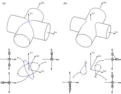
Any of the systems in (3)–(9) can now be written, and note that they can be solved analytically in this case. For example, if L1 =L2 = 1, the C-space has a single connected compo-nent composed of two ellipses intersecting on thexC axis [see
Fig. 2(a)], and the solutions of the systems in (3) reveal that the singularity set has six isolated configurations, marked in red in Fig. 2(a) bottom, with the following values ofq:
(a) (b)
Fig. 2. Configuration space (in blue) and singularities (red dots) of the three-slider mechanism for (a)L1=L2and (b)L1> L2with some examples of singular configurations depicted. In this mechanism, the configuration space corresponds to the intersection of two cylinders at right angles.
All of these configurations satisfy both systems in (3) so that both the FIKP and the IIKP are indeterminate in them. It turns out, moreover, that the four configurations withxC = 0satisfy
the systems in (6)–(8), meaning that they are both singularities belonging to each of the IO, II, and RPM types. Each of the other two configurations, which lie on thexC axis, is a singularity of
RI, RO, and RPM types, because it satisfies the systems (4), (5), and (9). These two configurations are in fact C-space sin-gularities, i.e., points where the tangent space is ill defined. The C-space self-intersects at these points and presents a bifurcation that allows a change in the mode of operation from both sliders moving on the same side of the horizontal axis,yAyB ≥0, to
one slider moving on each side,yAyB ≤0.
The topology of the C-space changes whenL1=L2. It no longer presents any bifurcation and is instead formed by two connected components [see Fig. 2(b)]. By solving (3) forL1 = 1 andL2 =0.8, for example, eight singularities are obtained:
(1,0.8,0), (−1,−0.8,0), (1,−0.8,0), (−0.6,0,0.8) (−1,0.8,0), (0.6,0,−0.8), (0.6,0,0.8), (−0.6,0,−0.8).
As before, each configuration withxC = 0is a singularity of
IO, II, and RPM types, while the other four configurations all belong to each of the RO and II types. There are no IIM-type singularities. In this case, to change the operation mode from
yA≥0toyA ≤0, the mechanism has to be disassembled.
It must be noted that if a singularity identification were at-tempted by means of an input–output velocity equation, for in-stance,yAvA =yBvB, which holds for all configurations, then
the singularities withxC = 0would not be detected.
V. ISOLATING THESINGULARITYSETS
A. Equation Formulation
In order to formulate the equations, note that the structure of all systems in (3)–(9) is very similar. The first line is always (1), because all solution points must correspond to feasible config-urations of the manipulator. The second line always involvesL or one of its submatrices, and the third line constrains the norm of some vector. For a manipulator that involves nonhelical lower pairs, the formulation proposed in [25] makes (1) directly adopt the form of a polynomial system of quadratic equations and al-lows writing the components ofLusing linear terms only [23]. Thus, the second equation of all systems will be quadratic as well, and the third equation is directly a quadratic expression. The helical pair could also be treated using the developments in [25], but its treatment is here omitted for ease of explanation. Written in the previous way, any one of the systems only involves monomials of the formxi, x2i, orxixj, wherexiand
xj refer to any two of their variables. Thus, by introducing
changes of variables of the formxk =x2i andxl =xixj, it is
possible to expand the systems into the form
Λ(x) =0 Γ(x) =0
(11)
wherexis a vector encompassing the variables of the original system and the newly introducedxkandxlones,Λ(x) =0is a
collection of linear equations inx, andΓ(x) =0is a collection
of scalar quadratic equations In the systems of (4)–(7), there is a vector that must be different from zero, but since the technique can also handle nonstrict inequalities as explained later, this latter condition can be enforced by setting
Ωa2 ≥ǫ (12)
for systems (4) and (7), and
Ωo2 ≥ǫ (13)
for systems (5) and (6), whereǫis a sufficiently small value. By using these inequalities, whose terms are also quadratic, some singularities might be overlooked, butǫcan be made arbitrarily small, reducing the set of missed solutions to a negligible size.
B. Initial Bounding Box
It can be shown that all variables in the systems can only take feasible values within bounded intervals. For example, from the results in [25], one can readily define such intervals for the variables inq, and the vector in the last line of each system has all of its components in the range[−1,1]. In the case of (6), the feasibility intervals for the entries ofΩo∗can be readily obtained
by mapping the known intervals usingAT
ou=Ωo∗, whereAois
formed by the columns ofLcorresponding to the output velocity vector. A similar mapping, but using the columns of the input velocity, allows the determination of feasibility intervals for
Ωa∗
in (7). Finally, by propagating the intervals of the previous variables through the expressionsxk =x2i andxl =xixj, it is
straightforward to define bounded intervals for thexk andxl
variables.
(a) (b)
Fig. 3. Polytope bounds within boxBcfor (a) parabola and for (b) hyperbolic
paraboloid.
In conclusion, from the Cartesian product of all such intervals, it is possible to define an initial boxBbounding the location of all pointsxsatisfying (11).
C. Numerical Solution
The algorithm for solving (11), together with (12) or (13) in the case of (4)–(7), applies two operations onB: boxshrinking
and boxsplitting. Using box shrinking, portions ofBcontaining no solution are eliminated by narrowing some of its defining intervals. This process is repeated until either 1) the box is found to contain no solution and is marked asempty, 2) the box is “sufficiently” small and can be considered asolutionbox, or 3) the box cannot be “significantly” reduced. In the latter case, the box is bisected via box splitting, and the whole process is recursively applied to the resulting subboxes until all box sides are below a given thresholdσ.
The crucial operation in this scheme is box shrinking, which is implemented as follows. The solutions falling in some subbox
Bc⊆ Bmust lie in the linear variety defined byΛ(x) =0. Thus,
we may shrinkBc to the smallest possible box bounding this variety insideBc. The limits of the shrunk box along dimension
xican be found by solving the linear programs
LP1: Minimizexi, subject to:Λ(x) =0,x∈ Bc
LP2: Maximizexi, subject to:Λ(x) =0,x∈ Bc.
However, observe that Bc can be further reduced because the solutions must also satisfy all equationsxk =x2i andxl =xixj
inΓ(x) =0. These equations can be taken into account by using
their linear relaxations [25]. Note that, if [vi, ui] denotes the
interval ofBcalong dimensionxi, then we have the following.
1) The portion of the parabolaxk =x2i lying inside Bc is
bound by the triangleA1A2A3, whereA1 andA2 are the points where the parabola intercepts the linesxi=viand
xi=ui, andA3is the point where the tangent lines atA1 andA2 meet [see Fig. 3(a)].
2) The portion of the hyperbolic paraboloidxl =xixj lying
insideBcis bound by the tetrahedronB1B2B3B4, where the pointsB1, . . . , B4are obtained by lifting the corners of the rectangle[vi, ui]×[vj, uj]vertically to the paraboloid
[see Fig. 3(b)].
Fig. 4. Progression of the numerical algorithm on computing the configuration space of the three-slider mechanism forL1=L2. From left to right, the sequence shows four stages of the computation, with the computed singularities of the mechanism shown overlaid in the right plot (in red). The method provided in this paper allows computing such boxes directly, without needing to isolate the whole configuration space. The boxes were magnified for clarity, because the box shrinking process yields too small boxes to be discerned.
linear programs is found unfeasible. In this step, the inequalities needed to model the conditions in (12) or (13) can also be taken into account by adding them to the linear programs.
As it turns out, the previous algorithm explores a binary tree of boxes whose internal nodes correspond to boxes that have been split at some time and whose leaves are either solution or empty boxes. The collectionBof all solution boxes is returned as output, and it is said to form a box approximation of the singularity set, because it forms a discrete envelope of the set whose accuracy can be adjusted through theσparameter. Notice that the algorithm is complete, in the sense that it will succeed in isolating all solution points accurately, provided that a small-enough value forσis used.
The application of the method to the three-slider mechanism can be seen in Fig. 4, which shows box approximations of the C-space in blue color, which are obtained by applying the method to (10) only. The red boxes correspond to singular configurations obtained by solving the systems in (4)–(9).
D. Computational Cost
The computational cost of the algorithm can be evaluated by analyzing the cost of one iteration, and the number of iterations to be performed, both in terms of the number of bodies (nb)
and joints (nj) of the manipulator. On the one hand, we can
consider that an iteration includes the box shrinking process for a given box. This involves solving2nx linear programs, where
nxis the number of variables in (11). Sincenxdepends linearly
on nb andnj, and Karmarkar’s bound for the complexity of
linear programming isO(n3x.5)[29], we can conclude that the cost of one iteration is worst-case polynomial innbandnj. On
the other hand, it is difficult to predict how many iterations will be required to isolate all solutions. The number of iterations largely depends on the chosenσ, as well as on the dimensiond
of the singularity subset considered. Ford= 0, the algorithm is quadratically convergent in the vicinity of the roots. Ford≥1, the cost is inversely proportional toσin the best case. For a fixed
σ, however, the amount of solution boxes grows exponentially withdso that an initial guess on the execution time is usually made on the basis ofdonly. The value ofdcan be estimated
TABLE II
PERFORMANCEDATA ON THEREPORTEDTESTCASES
by noting that the singularity set is typically of codimension one relative to the C-space and using the Gr¨ubler–Kutzbach formula on nb and nj to determine the C-space dimension.
Detailed properties of the algorithm, including an analysis of its completeness, correctness, and convergence order, are given in [25].
VI. TESTCASES
The performance of the approach is next illustrated in two test cases. The results were obtained using a parallelized version of the method implemented in C [30]. Table II summarizes the main performance data on the various singularity sets analyzed. For each set, we indicate its dimension (d), the number of equations (Neq) and variables (Nvar) in its defining system, the number of solution boxes returned by the method (Nb oxes), the accuracy threshold assumed (σ), theǫparameter where applicable, and the time required to compute the set (t), in seconds, on a Xeon processor grid able to run 160 threads in parallel.
A. Planar Manipulator
Fig. 5. Two-degree-of-freedom planar manipulator. The link dimensions are
AB=AD=B C=DE= 1, C D=F G= 2, C G=1.5, andE F = 3.
follows:
cosθA+ cosθB −2 cosθD −1 = 0 sinθA+ sinθB−2 sinθD = 0 2 cosθD+32cosθC + 2 cosθG −3 cosθE −1 = 0 2 sinθD+32sinθC + 2 sinθG−3 sinθE = 0 −x+ 2 cosθD+32cosθC = 0 −y+ 2 sinθD+32sinθC = 0
⎫ ⎪ ⎪ ⎪ ⎪ ⎪ ⎪ ⎪ ⎪ ⎪ ⎬
⎪ ⎪ ⎪ ⎪ ⎪ ⎪ ⎪ ⎪ ⎪ ⎭
(14)
where θA, θB, θC, θD, θE, andθG are the counterclockwise
angles of linksAB, BC, CG, DC, EF, andGF, respectively, relative to the ground, andxandyare the coordinates of point
Grelative to a fixed frame centered inD. The velocity equa-tion of the manipulator may now be obtained by differentiating (14) with respect to all variables, but it could also be obtained using the twist loop equations, or by any other means. In or-der to achieve the desired quadratic formulation, the changes of variablescτ = cosθτ andsτ = sinθτ can now be applied
for allτ ∈ {A, B, C, D, E, G}. Since the variablescτ andsτ
represent the cosine and sine of a variable, the circle equations
c2
τ +s2τ = 1 also need to be introduced into the systems for
every angleθτ.
Given that the manipulator has two degrees of freedom, its configuration space is a surface, which is shown projected onto thex, y, andθA variables in Fig. 6. This surface was obtained
from the computation of all solutions of (1) using the same numerical technique presented in the previous section. Note that by fixingx, y, andθA, there are still two possible positions of
pointFso that most of the points in this projection correspond, in fact, to two different configurations of the manipulator. Only the points whereE, F, andG are aligned represent a single configuration, and these are exactly the boundaries of the two “holes” that the surface presents.
The singularity set is generally of lower dimension than the configuration space so that only curves or points are to be ex-pected in the solution set of all systems of equations. The result of the computation of each singularity type is shown in Figs. 7 and 8, projected onto the output and one input (x, y, θA), and
onto the output only, respectively. In Fig. 7, the configuration space is shown in blue, separated in two parts so that a cross
Fig. 6. 2-D configuration space of the manipulator in Fig. 5 computed at
σ=0.1. Two holes can be seen, whose boundary corresponds to configurations whereE , F, andGare aligned.
section can be seen, but both parts are actually connected throughπand−π, as shown in Fig. 6. The gray area in Fig. 8 represents all attainable positions of pointG, i.e., the workspace of the manipulator.
As it turns out, this manipulator contains no IIM configura-tions, and the computation of this type of singularity gives no box as output. On the contrary, there are eight distinct RPM singularities, which in these projections appear coincident in pairs as four orange boxes, corresponding to the two possible locations ofF. Using a different projection, for instance, onto (θA, θE, θD), the eight boxes appear separated.
The green curves correspond to singularities that are of both the RI and IO types. These configurations can be seen to contour the two “holes” of the configuration space in this projection. The red curves correspond to configurations simultaneously belong-ing to the RO and II types. Even if the curves for RI and IO seem to coincide everywhere, there are some IO configurations that are not of RI type, and the same happens for II and RO singularities, respectively. This is illustrated in Fig. 7 with a closeup on the left that shows only the output of computing RI singularities. These gaps on the curves of RI and RO, which can be found by properly adjusting the ǫparameter, coincide with the location of the RPM singularities, and hence, the RPM singularities are also of II and IO types (but not of RI or RO types). Fig. 8(a) shows an example of an (RPM, II, IO) singu-larity, while Fig. 8(b) and (c) shows examples of (RI, IO) and (RO, II) singularities, respectively.
Fig. 7 also shows yellow (arcs of) curves that correspond to configurations where pointsD, B, andGare aligned. For each yellow-marked triple (x, y, θA), withD, B, andGcollinear,
there are two possible locations of pointC. In contrast, pointC
is uniquely determined for any other (x, y, θA). Thus, a point
Fig. 7. Singular configurations of the mechanism in Fig. 5 shown overlaid onto a projection of its configuration space. Different colors are used to identify the several singularity types encountered: green for the RI and IO types, red for the RO and II types, and orange for the RPM type.
Fig. 8. Projection of the plot in Fig. 7 to the(x, y)plane. (a) Singularity of RPM, IO, and II types. (b) Singularity of RI and IO types. (c) Singularity of RO and II types.
theprojectionof the configuration space on the (x, y, θA) space.
The four configurations for each point can be identified with the two sides (“in” and “out”) of the two sheets that intersect. The configuration space itself has no self-intersections as there are no configuration space, or IIM-type, singularities. The yellow points are only singularities of the projection map. The four or-ange vertices of the yellow curve arcs in Fig. 7 correspond to the eight configurations whereD, B, G, andCare collinear. These are the mechanism’s RPM-type singularities. They are branch-ing points for the inverse kinematics solution, because pointC
can move in two different ways out of such a configuration. The
other configurations where the working mode changes are those whereE, F, andGare aligned.
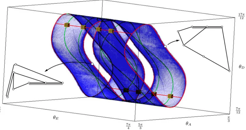
Using the same color code, Figs. 9 and 10 show the projection of the results onto the 3-D space of the two input angles and one passive joint angle (θA, θE, θD) and onto the 2-D input
space only. The eight RPM singularities appear separated. As before, for fixed values ofθA, θE, andθD, there are still two
Fig. 9. Projection of the configuration space and the computed singularities to the(θA, θE, θD)space, together with two configurations whereC, G, andFare
aligned. Green corresponds to the RI and IO types, red to the RO and II types, and orange to the RPM type. There are no singularities of IIM type.
Fig. 10. Projection of the plot in Fig. 9 to the(θA, θE)space.
of those configurations whereG, C, andFare aligned and there is only one possibility forC. Note that none of these “holes” coincides with one in the previous projection; however, once again, crossing each curve allows the transition between two different working modes. One can imagine the two working modes as the two “sides” of the surface of the configuration-space projection. To “get to the opposite side,” i.e., to change working mode, the motion curve must “go through a hole.”
B. Spatial Manipulator
To illustrate the method on a spatial manipulator, we next apply it to the Stewart–Gough platform. For the sake of con-ciseness, we concentrate on computing the forward singularity locus only, which is the most relevant and representative of the kind of complexity to be confronted in the spatial case. This
amounts to formulating and solving the left system in (3) using the proposed approach.
The platform consists of a moving plate connected to a fixed base by means of six legs, where each leg is a universal-prismatic-spherical chain (see the left side of Fig. 11). The six prismatic joints are actuated, allowing to control the six de-grees of freedom of the platform, and the remaining joints are passive [31].
The assembly constraints can be formulated as follows. Let
Ai andBi be the center points of the universal and spherical
joints. Let alsoF1andF2be fixed and mobile reference frames, centered inOandP, respectively. Then, the constraints imposed by each leg on the moving plate can be written as
pF1 =aF1
i +didFi1 −Rb F2
i (15)
dF1
i
2 = 1
(16)
where pF1,aF1
i , and b F2
i are the position vectors of points
P, Ai, andBi in the indicated frames, anddFi1 is a unit vector
along the ith leg, expressed in frame F1. In addition, di is
the length of the leg, which represents the displacement of the prismatic joint, and Ris the rotation matrix that provides the orientation of F2 relative toF1. The pose of the platform is given by(pF1,R).
In this case, (1) is the system formed by (15) and (16) for all legs, together with the conditions
s2 = 1, s·t= 0
t2 = 1, s×t=w
i
that forceR= [s,t,w]to represent a valid rotation.
The velocity equation can be obtained by writing the expres-sion of the output twistTˆfollowing each leg
ˆ
T = Ωa iSˆai +
5
j= 1
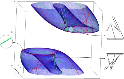
Fig. 11. (Left) Stewart–Gough platform. (Center and right) Slices of its forward singularity set for a constant orientation given byφ=−2◦, θ= 30◦, and ψ=−87◦, and for the fixed positionpF1 = [10,10,10]T. The position and orientation variables of the platform have been limited to the ranges[−100,100]and
[−90◦,90◦], respectively.
whereSˆa
i and theSˆ p
i,j are the unit twists of the active and the
five passive joints of theith leg, respectively. By gathering (17) for all legs, we obtain a 36×42 matrixL, and a velocity vector m containing the six components of the output twist, the six active velocities of the prismatic joints, and the 30 passive joint velocities of the universal and spherical joints. This results in a relatively large system of equations, but by multiplying each side of (17) by a unit screw reciprocal to all passive joint twists of the leg, we can conclude that the forward singularities are the configurations for which the conventional screw JacobianJ is singular [18], [32]. This condition is advantageous becauseJis only 6×6, and generally produces a much smaller system.
For some configurations, the space of reciprocal screws of a given leg may be of dimension larger than one, and (17) should be multiplied by a whole basis of reciprocal screws of the leg [33]. In the Stewart–Gough platform, this can only happen when the center of the leg’s spherical joint is in the plane of the two revolute-joint axes of the universal joint, which result in a singularity of RPM type. Since joint limits and other constraints typically exclude such singularities in real platforms, we will not compute them here.
Two slices of the forward singularity locus are shown in Fig. 11, computed at a constant orientation and at a constant po-sition of the platform. Alternative slices could also be obtained if desired, simply by fixing a different set of pose parameters. The geometric dimensions assumed here correspond to the aca-demic manipulator studied in [6]. The Euler anglesφ, θ, andψ
are those for whichR=Rz(ψ)Ry(θ)Rx(φ), which also
coin-cide with the ones assumed in [6]. From the results in Table II, we note that it is computationally much harder to compute the constant position slice. This agrees with the fact that the sys-tem to be solved is much larger, and its equations are highly nonlinear, in comparison with those of the constant orientation slice.
VII. CONCLUSION
This paper has proposed a method for the numerical compu-tation and detailed classification of the entire singularity set of a lower-pair manipulator with arbitrary geometry. Systems of equations have been defined to compute the set, and each one
of the singularity subsets has been identified in [18]. To solve any of the systems, a numerical method that is based on linear relaxations has been proposed, which can obtain a box approx-imation of the solution set with the desired accuracy, even in the presence of self-intersections or dimension changes in the set [23], [34]. The approach is based on a recursive segmentation and reduction of the search space and is particularly practical and useful on low degree-of-freedom manipulators like the one in Section VI-A. This example has been chosen for its high il-lustrative value, since it allows a clear analysis and presentation of the results in a moderate-dimensional case. It also shows how complex can be the topology of the configuration space and its singularity-induced partitions. As demonstrated in Section VI-B, the analysis of manipulators with higher dimensional singu-larity sets does not add fundamental difficulties to the method, other than increasing the computation times, as with any other method. The detailed interpretation and visualization of the sin-gularity sets of these and other manipulators will be the subject of future work. Additional work is envisaged to also extend the developments to deal with redundant manipulators [18], [35].
REFERENCES
[1] C. Gosselin and J. Wang, “Singularity loci of a special class of spherical three-degree-of-freedom parallel mechanisms with revolute actuators,”
Int. J. Robot. Res., vol. 21, no. 7, pp. 649–659, 2002.
[2] I. A. Bonev. (2002). “Geometric analysis of parallel mechanisms,” Ph.D. dissertation, Facult´e des Sciences et de G´enie, Univ. de Laval. [Online]. Available:http://goo.gl/lKhw6
[3] I. A. Bonev, D. Zlatanov, and C. Gosselin, “Singularity analysis of 3-DOF planar parallel mechanisms via screw theory,”ASME J. Mech. Design, vol. 125, pp. 573–581, 2003.
[4] I. Ebert-Uphoff, J. Lee, and H. Lipkin, “Characteristic tetrahedron of wrench singularities for parallel manipulators with three legs,”Proc. Inst. Mech. Eng. C, J. Mech. Eng. Sci., vol. 216, no. 1, pp. 81–93, 2002. [5] J. Wang and C. Gosselin, “Singularity loci of a special class of spherical
3-DOF parallel mechanisms with prismatic actuators,”ASME J. Mech. Design, vol. 126, no. 2, pp. 319–326, 2004.
[6] H. Li, C. Gosselin, M. Richard, and B. St-Onge, “Analytic form of the six-dimensional singularity locus of the general Gough-Stewart platform,”
ASME J. Mech. Design, vol. 128, pp. 279–288, 2006.
[7] I. A. Bonev and C. Gosselin, “Analytical determination of the workspace of symmetrical spherical parallel mechanisms,” IEEE Trans. Robot., vol. 22, no. 5, pp. 1011–1017, Oct. 2006.
[9] J.-P. Merlet, “A formal-numerical approach for robust in-workspace sin-gularity detection,”IEEE Trans. Robot., vol. 23, no. 3, pp. 393–402, Jun. 2007.
[10] D. Kanaan, P. Wenger, S. Caro, and D. Chablat, “Singularity analysis of lower mobility parallel manipulators using Grassmann–Cayley algebra,”
IEEE Trans. Robot., vol. 25, no. 5, pp. 995–1004, Oct. 2009.
[11] J. Schadlbauer and M.-L. Husty, “A complete analysis of the 3-RPS manipulator,” inMachines and Mechanism. New Delhi, India: Narosa, 2011, pp. 410–419.
[12] J. Borr`as, F. Thomas, and C. Torras, “Singularity-invariant families of line-plane 5-SPU platforms,”IEEE Trans. Robot., vol. 27, no. 5, pp. 837–848, Oct. 2011.
[13] M.-L. Husty, J. Schadlbauer, S. Caro, and P. Wenger, “Self-motions of 3-RPS manipulators,”New Trends Mech. Mach. Sci., Theory Appl. Eng., vol. 7, pp. 121–130, 2012.
[14] C. Gosselin and J. Angeles, “Singularity analysis of closed-loop kine-matic chains,”IEEE Trans. Robot. Autom., vol. 6, pp. 281–290, Jun. 1990.
[15] D. Zlatanov, R. Fenton, and B. Benhabib, “Singularity analysis of mecha-nisms and robots via a motion-space model of the instantaneous kinemat-ics,” inProc. IEEE Int. Conf. Robot. Autom., 1994, pp. 980–985. [16] D. Zlatanov, R. Fenton, and B. Benhabib, “A unifying framework for
classification and interpretation of mechanism singularities,”ASME J. Mech. Design, vol. 117, pp. 566–572, 1995.
[17] D. Zlatanov, B. Benhabib, and R. Fenton, “Identification and classifica-tion of the singular configuraclassifica-tions of mechanisms,”Mech. Mach. Theory, vol. 33, pp. 743–760, 1998.
[18] D. Zlatanov. (1998). “Generalized singularity analysis of mechanisms,” Ph.D. dissertation, Univ. Toronto, Toronto, ON, Canada. [Online]. Avail-able: http://goo.gl/rnAUy
[19] F. Park and J. Kim, “Singularity analysis of closed kinematic chains,”
ASME J. Mech. Design, vol. 121, pp. 32–38, 1999.
[20] O. Bohigas, D. Zlatanov, L. Ros, M. Manubens, and J. M. Porta, “Numer-ical computation of manipulator singularities,” inProc. IEEE Int. Conf. Robot. Autom., 2012, pp. 1351–1358.
[21] O. Bohigas, M. Manubens, and L. Ros, “Singularities of non-redundant manipulators: A short account and a method for their computation in the planar case,”Mech. Mach. Theory, vol. 68, pp. 1–17, 2013.
[22] J. G. De Jal´on and E. Bayo,Kinematic and Dynamic Simulation of Multi-body Systems. New York, NY, USA: Springer-Verlag, 1993.
[23] O. Bohigas. (2013). “Numerical computation and avoidance of manip-ulator singularities,” Ph.D. dissertation, Univ. Polit`ecnica de Catalunya, Barcelona, Spain. [Online]. Available:http://goo.gl/wlR0i
[24] J. Selig,Geometric Fundamentals of Robotics. New York, NY, USA: Springer-Verlag, 2005.
[25] J. M. Porta, L. Ros, and F. Thomas, “A linear relaxation technique for the position analysis of multi-loop linkages,”IEEE Trans. Robot., vol. 25, no. 2, pp. 225–239, Apr. 2009.
[26] O. Bohigas, M. Manubens, and L. Ros, “A complete method for workspace boundary determination on general structure manipulators,”IEEE Trans. Robot., vol. 28, no. 5, pp. 993–1006, Oct. 2012.
[27] C. W. Wampler and A. J. Sommese, “Applying numerical algebraic geom-etry to kinematics,” in21st Century Kinematics. New York, NY, USA: Springer-Verlag, 2013, pp. 125–160.
[28] D. Cox, J. Little, and D. O’Shea,An Introduction to Computational Al-gebraic Geometry and Commutative Algebra, 3rd ed. New York, NY, USA: Springer-Verlag, 2007.
[29] N. K. Karmarkar, “A new polynomial-time algorithm for linear program-ming,”Combinatorica, pp. 373–395, 1984.
[30] J. M. Porta, L. Ros, O. Bohigas, M. Manubens, C. Rosales, and L. Jaillet, “The CUIK suite: Motion analysis of closed-chain multibody systems,”
IEEE Robot. Autom. Mag., 2013, in press.
[31] J.-P. Merlet,Parallel Robots. New York, NY, USA: Springer-Verlag, 2006.
[32] K. J. Waldron and K. H. Hunt, “Series-parallel dualities in actively coor-dinated mechanisms,”Int. J. Robot. Res., vol. 10, pp. 473–480, 1991. [33] D. Zlatanov, R. Fenton, and B. Benhabib, “Analysis of the instantaneous
kinematics and singular configurations of hybrid-chain manipulators,” in
Proc. ASME 23rd Biennial Mech. Conf., 1994, vol. 72, pp. 467–476. [34] O. Bohigas, D. Zlatanov, M. Manubens, and L. Ros, “On the numerical
classification of the singularities of robot manipulators,” inProc. ASME Int. Design Eng. Tech. Conf., 2012, pp. 1287–1296.
[35] A. M¨uller, “On the terminology and geometric aspects of redundant par-allel manipulators,”Robotica, vol. 31, no. 1, pp. 137–147, 2013.
Oriol Bohigas received the double M.S. degree in mechanical engineering from the Universitat Polit`ecnica de Catalunya (UPC), Barcelona, Spain, and in aeronautical engineering from the Institut Sup´erieur de l’A´eronautique et de l’Espace (ISAE), Toulouse, France, in 2006. In 2013, he received the Ph.D. degree in robotics from the UPC.
After a research internship with Airbus France, Toulouse, he worked for two years as a Space Engineer with the Centre National d’Etudes Spa-tiales, Toulouse. He is currently with the Kinemat-ics and Robot Design Group, the Institut de Rob`otica i Inform`atica Industrial, Barcelona. His research interests include workspace and singularity analysis of robot mechanisms.
Dimiter Zlatanovreceived the Diploma in mathe-matics and mechanics from the University of Sofia, Sofia, Bulgaria, in 1989 and the Ph.D. degree in me-chanical engineering from the University of Toronto, Toronto, ON, Canada, in 1998.
He has held positions with Laval University, Que-bec City, QC, Canada; the University of Innsbruck, Innsbruck, Austria; and Tokyo City University, Seta-gaya, Japan. He is currently on the faculty with the Department of Mechanical and Energy Engineering, University of Genoa, Genoa, Italy. His research inter-ests include the design, kinematics, dynamics and control of mechanisms and robotic systems.
Llu´ıs Rosreceived the mechanical engineering de-gree in 1992 and the Ph.D. dede-gree (Hons.) in indus-trial engineering in 2000, both from the Universitat Polit`ecnica de Catalunya, Barcelona, Spain.
From 1993 to 1996, he worked with the Con-trol of Resources Group, Institut de Cibern`etica, Barcelona. He was a Visiting Scholar with York University, Toronto, ON, Canada, in 1997; the Uni-versity of Tokyo, Tokyo, Japan, in 1998; and the Laboratoire d’Analyse et Architecture des Syst`emes, Toulouse, France, in 1999. He joined the Institut de Rob`otica i Inform`atica Industrial, Barcelona, in 1997, where he has been an Associate Researcher with the Spanish National Research Council since 2005. His research interests include geometry and kinematics, with applications to robotics, computer graphics, and machine vision.
Montserrat Manubens received the degree in mathematics from the Universitat de Barcelona, Barcelona, Spain, in 2001 and the Ph.D. degree (Hons.) in computer algebra from the Universitat Polit`ecnica de Catalunya, Barcelona, in 2008.
From 2009 to 2010, she worked with the Robotics Group, Institut de Recherche en Communications et Cybern´etique de Nantes, Nantes, France, in the anal-ysis of cuspidal robots. Since 2011, she has been a Juan de la Cierva contractor with the Institut de Rob`otica i Inform`atica Industrial, Barcelona. Her cur-rent research interests include mathematics and kinematics, with applications to robotics.
Josep M. Porta received the engineering degree in computer science in 1994 and the Ph.D. degree (Hons.) in artificial intelligence in 2001, both from the Universitat Polit`ecnica de Catalunya, Barcelona, Spain.

![Fig. 2(a)], and the solutions of the systems in (3) reveal that the](https://thumb-ap.123doks.com/thumbv2/123dok/3536605.1444045/4.594.302.528.533.620/fig-solutions-systems-reveal.webp)


![Fig. 11.(Left) Stewart–Gough platform. (Center and right) Slices of its forward singularity set for a constant orientation given by φ = −2◦, θ = 30◦, andψ = −87◦, and for the fixed position pF1 = [10, 10, 10]T](https://thumb-ap.123doks.com/thumbv2/123dok/3536605.1444045/11.594.84.515.66.205/stewart-platform-center-slices-singularity-constant-orientation-position.webp)
