Modul 5
Pemilihan Bahan & Proses
Topik 4 :
Diagram Seleksi Material
Versi 1.0
Disarikan dari buku :
Ashby, M.F. : “Material Selection in Mechanical Design”, Pergamon Press, 1992.
Oleh:
R. Ariosuko Dh.
Email:[email protected]
© 2008
Teknik Mesin
Fakultas Teknik Universitas Mercu Buana
disusun pertama : Dzulhijjah 1423 H
BAB 4
Diagram Seleksi Material
4.1. Intro dan Sinopsis
4.2. Displai Properti Material Properties 4.3. Diagram-diagram Properti Material 4.4. Rangkuman dan Kesimpulan 4.5. Bacaan lanjut
4.6. Evaluasi
4.1 Intro dan Sinopsis
Properti material membatasi performa. Tetapi jarang performa suatu komponen
tergantung pada hanya pd satu properti saja. Melainkan hampir selalu
merupakan suatu kombinasi (atau beberapa kombinasi) properti, yang berarti:
orang berpikir, sebagai contoh, tentang nisbah strength-to-weight ( sf/r ), atau
nisbah stiffness-to-weight ( E/r ), yang mana masuk disain kelas ringan. Ini melahirkan gagasan untuk merencanakan satu properti terhadap yang lain,
merencanakan daerah di dalam ruang properti yang diduduki oleh
masing-masing kelas material, dan sub-daerah yang diduduki oleh material secara
individu.
The idea of a materials selection chart-is described briefly in Section 4.2.
Section 4.3 is not so brief: it introduces, the charts themselves. There is no
need to read it all, but it is helpful to persist far enough to be able to read and
interpret the charts fluently, and to understand what the additional contours
mean. If, later, you use one chart a lot, you should read the background to it,
given here, to be sure of interpreting it correctly.
A compilation of all the charts, with a brief explanation of each, is contained in
Appendix C. It is intended for reference — that is, as a tool for tackling real
design problems.
Each property of an engineering material has a characteristic range of values.
The range is large: of the properties considered here — properties such as
modulus, toughness, thermal conductivity — most have values which span
roughly five decades.
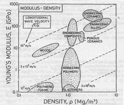
Gb. 4.1 Ide diagram properti material; modulus Young, E, diplot thd density, ρ, pd skala logarithmic. Setiap klas material mewakili suatu bagian unik tertentu pd diagram. Skala logarithmic memungkinkan kecepatan
gelombang longitudinal elastik ν = (E/ρ)1/2 utk diplot sbg suat set permukaan paralel.
The values are conveniently displayed on material selection charts, illustrated by Fig. 4.1. One property (the modulus, E, in this case) is plotted against another (the density, p) on logarithmic scales. The range of the axes is chosen to
include all materials, from the lightest, flimsiest foams to the stiffest, heaviest
metals. It is then found that data for a given class of materials (polymers, for
example) cluster together on the chart; the subrange associated with one material class is, in all cases, much smaller than the full range of that property. Data for one class can be enclosed in a property envelope, as shown in Fig. 4.1.
The envelope encloses all members of the class.
All this is simple enough — just a helpful way of plotting data. But by choosing
the axes and scales appropriately, more can be added. The speed of sound in a
solid depends on the modulus, E and the density, p; the longitudinal wave speed v, for instance, is
=
E
1/2
log E = log ρ + 2 log v
For a fixed value of v, this equation plots as a straight line of slope 1 on Fig. 4.1. This allows us to add contours of constant wave velocity to the chart: they are the family of parallel diagonal lines, linking materials in which longitudinal waves
travel with the same speed. All the charts allow additional fundamental
relationships of this sort to be displayed. And thereis more: design-optimising
Among the mechanical and thermal properties, there are eighteen which are of
primary importance, both in characterising the material, and in engineering
design. They were listed in Table 3.1: they include density, modulus, strength,
toughness, thermal conductivity, diffusivity and expansion. The charts display
data for these properties, for the nine classes of materials listed in Table 4.1.
The class list is expanded from the original six by distinguishing engineering composites from foams and from woods though all, in the most general sense, are composites; and by distinguishing the high-strength eng if leering ceramics
(like silicon carbide) from the low strength, porous ceramics (like brick). Within each class, data are plotted for a representative set of materials, chosen both to
span the full range of behaviour for the class, and to include the most common
and most widely used members of it. In this way the envelope for a class
encloses data not only for the materials listed in Table 4.1, but for virtually all
other members of the class as well.
The charts show a range of values for each property of each material;
sometimes the range is narrow: the modulus of copper, for instance, varies by
only a few percent about its mean value, influenced by purity, texture and such
like. Sometimes it is wide: the strength of alumina ceramic can vary by a factor
of 100 or more, influenced by porosity, grain size and so on. Heat treatment
and mechanical working have a profound effect on yield strength, damping and
the toughness of metals. Crystallinity and degree of cross-linking greatly
influence the modulus of polymers, and so on. These structure-sensitive
properties appear as elongated bubbles within the envelopes on the charts. A
bubble encloses a typical range for the value of the property for a single
material. Envelopes (heavier lines) enclose the bubbles for a class.
The data plotted on the charts have been assembled from a variety of sources,
the most accessible of which are listed under Further Reading, at the end of this
chapter.
4.3 Diagram properti material
The Modulus — Density Chart (Chart 1, Fig. 4.2)
these are effects of modulus. Lead is heavy; cork is buoyant: these are effects
of density. Figure 4.2 shows the full range of Young’s modulus, E, and density, p, for engineering materials.
Data for members of a particular class of materials cluster together and can be
enclosed by an envelope (heavy line). The same class envelopes appear on all
the diagrams: they correspond to the main headings in Table 4.1.
The density of a solid depends on three factors: the atomic weight of its atoms or ions, their size, and the way they are packed. The size of atoms does not
vary much: most have a volume within a factor of two of 2 x 10~ m3. Packing
fractions do not vary much either — a factor of 2, more or less: close-packing
gives a packing fraction of 0.74; open networks, like that of the diamond-cubic
structure, give about 0.34. The spread of density comes mainly from that of
atomic weight, from 1 for hydrogen to 238 for uranium. Metals are dense
because they are made of heavy atoms, packed densely; polymers have low
densities because they are largely made of carbon (atomic weight: 12) and
hydrogen in a linear, two- or three-dimensional network. Ceramics, for the most
part, have lower densities than metals because they contain light 0, N or C
atoms. Even the lightest atoms, packed in the most open way, give solids with a
density of around 1 Mg/rn3. Materials with lower densities than this are foams —
materials made up of cells containing a large fraction of pore space. The moduli
of most materials depend on two factors: bond stiffness, and the density of
bonds per unit area. A bond is like a spring: it has a spring constant, S (units:
N/rn). Young’s modulus, E, is roughly
E = S / r0 (4.1)
where r0 is the “atom size” (r ~ is the mean atomic or ionic volume). The wide range of moduli is largely caused by the range of values of S. The covalent
bond is stiff (S = 20—200 N/rn); the metallic and the ionic a little less so (S = 15 — 100 N/rn). Diamond has a very high modulus because the carbon atom is small (giving a high bond density) and its atoms are linked by very strong
springs (S = 200 N/rn). Metals have high moduli because close-packing gives a
diamond. Polymers contain both strong diamond-like covalent bonds and weak
hydrogen or Van der Waals bonds (S = 0.5 —2 N/rn); it is the weak bonds which stretch when the polymer is deformed, giving low moduli.
But even large atoms (r0 = 3 x l0~°m) bonded with weak bonds (S = 0.5 N/rn) have a modulus of roughly
E= 0,5
3x10⁻¹⁰ ≈ 1 GPa (4.2)
This is the lower limit for true solids. The chart shows that many materials have moduli that are lower than this: they are either elastomers, or foams.
Elastomers have a low E because the weak secondary bonds have melted (their glass temperature, T~, is below room temperature) leaving only the very weak “entropic” restoring force associated with tangled, long-chain molecules;
and foams have low moduli because the cell walls bend (allowing large
The chart shows that the modulus of engineering materials spans five decades,1
from 0.01 GPa (low density foams) to 1000 GPa (diamond); the density spans a
factor of 2000, from less than 0.1 to 20 Mg/m3. At the level of approximation of
interest here (that required to reveal the relationship between the properties of
materials classes) we may approximate the shear modulus, G, by 3E/8 and the bulk modulus, K, by E, for all materials except elastorners (for which G = E/3
and K>>E).
The log scales allow more information to be displayed. The velocity of elastic
1Very low density foams and gels (which can be thought of as molecular scale, fluid-filled, foams) can have
moduli far lower than this. As an example, gelatin (as in Jello) has a modulus of about 5 x 10⁻⁵ GPa. Their
waves in a material, and the natural vibration frequencies of a component made
of it, are proportional to (E/p)½; the quantity (EIp)½ itself is the velocity of longitudinal waves in a thin rod of the material. Contours of constant (E/p)½ are plotted on the chart, labelled with the longitudinal wave speed: it varies from
less than 50 rn/s (soft elastomers) to a little more than iO~ rn/s (fine ceramics).
We note that aluminium and glass, because of their low densities, transmit
waves quickly despite their low moduli. One might have expected the sound
velocity in foams to be low because of the low modulus; but the low density
almost compensates. That in wood, across the grain, is low; but along the grain,
it is high — roughly the same as steel — a fact made use of in the design of
musical instruments.
The chart helps in the common problem of material selection for applications in
which weight must be minimised. Guide lines corresponding to three common
geometries of loading are drawn on the diagram. They are used in the way
described in Chapters 5 and 6 to select materials for elastic design at minimum
weight.
The Strength — Density Chart (Chart 2, Fig. 4.3)
The modulus of a solid is a well-defined quantity with a sharp value. The
strength is not. The word “strength” needs definition (see also Chapter 3,
Section 3.3). For metals and polymers it is the yield strength, but since the range of materials includes those which have been worked, the range spans
initial yield to ultimate strength; for most practical purposes it is the same in
tension and compression. For brittle ceramics, it is the crushing strength in compression, not that in tension which is about fifteen times smaller; the envelopes for brittle materials are shown as broken lines as a reminder of this.
For elastomers, strength means the tear strength. For composites, it is the
tensile failure strength (the compressive strength can be less, because of fibre buckling).
Figure 4.3 shows these strengths, for which we will use the symbol O~ (despite
the different failure mechanisms involved), plotted against density, p. The
considerable vertical extension of the strength bubble for an individual material
reflects its wide range, caused by degree of alloying, work hardening, grain
can be enclosed in an envelope (heavy line). Each occupies a characteristic
area of the chart.
The range of strength for engineering materials, like that of the modulus, spans
energy-absorbing systems) to 104 MPa (the strength of diamond, exploited in
the diamond anvil press). The single most important concept in understanding
this wide range is that of the lattice resistance or Peierls stress: the intrinsic resistance of the structure to plastic shear. Plastic shear in a crystal involves the
motion of dislocations. Metals are soft because the non-localised metallic bond
does little to prevent dislocation motion, whereas ceramics are hard because
their more localised covalent and ionic bonds (which must be broken and
reformed when the structure is sheared), lock the dislocations in place. In
non-crystalline solids we think instead of the energy associated with the unit step of
the flow process: the relative slippage of two segments of a polymer chain, or
the shear of a small molecular cluster in a glass network. Their strength has the
same origin as that underlying the lattice resistance: if the unit step involves
breaking strong bonds (as in an inorganic glass), the material will be strong; if it
only involves the rupture of weak bonds (the Van de Waals bonds in polymers
for example), it will be weak. Materials which fail by fracture do so because the
lattice resistance or its amorphous equivalent is so large that fracture happens
first.
When the lattice resistance is low, the material can be strengthened by
introducing obstacles to slip: in metals, by adding alloying elements, particles,
grain boundaries and even other dislocations (“work hardening”); and in
polymers by cross-linking or by orienting the chains so that strong covalent as
well as weak Van der Waals bonds are broken. When, on the other hand, the
lattice resistance is high, further hardening is superfluous — the problem
becomes that of suppressing fracture (next section).
An important use of the chart is in materials selection in lightweight plastic
design. Guidelines are shown for materials selection in the minimum weight
design of tics, columns, beams and plates, and for yield-limited design of
moving components in which inertial forces are important. Their use is
described in Chapters 5 and 6.
The Fracture Toughness — Density Chart (Chart 3, Fig. 4.4)
Increasing the plastic strength of a material is useful only as long as it remains
crack is measured by the fracture toughness, KIc. It is plotted against density
in Fig. 4.4. The range is large: from 0.01 to over 100 MPa m1/2 . At the lower end
of this range are brittle materials which, when loaded, remain elastic until they
fracture. For these, linear elastic fracture mechanics works well, and the
fracture toughness itself is a well-defined property. At the upper end lie the
super-tough materials, all of which show substantial plasticity before they break.
For these the values of KIcare approximate, derived from critical J-integral (Jc)
and critical crack-opening displacement (dc) measurements (by writing KIc =
(EJc)½, for instance). They are helpful in providing a ranking of materials. The
guidelines for minimum weight design are explained in Chapter 5. The figure shows one reason for the dominance of metals in engineering: they almost all
have values of KIcabove 20 MPa m½, a value often quoted as a minimum for
The Modulus — Strength Chart (Chart 4, Fig. 4.5)
High-tensile steel makes good springs. But so does rubber. How is it that two
such different materials are both suited for the same task? This and other
questions are answered by Fig. 4.5, the most useful of all the charts.
It shows Young’s modulus, E, plotted against strength, o~. The qualifications on “strength” are the same as before: it means yield strength for metals and
polymers, compressive crushing strength for ceramics, tear strength for
elastomers, and tensile strength for composites and woods; the symbol o,is
used for them all. The ranges of the variables, too, are the same. Contours of
normailsed strength, c1/E, appear as a family of straight parallel lines.
Examine these first. Engineering polymers have normalised strengths between
0.01 and 0.1. In this sense they are remarkably strong: the values for metals are
at least a factor of 10 smaller. Even ceramics, in compression, are not as
strong, and in tension they are far weaker (by a further factor of 15 or so).
Composites and woods lie on the 0.01 contour, as good as the best metals.
Elastomers, because of their exceptionally low moduli, have values of oj/E
larger than any other class of material: 0.1 to 10.
The distance over which interatomic forces act is small — a bond is broken if it
is stretched to more than about lOWo of its original length. So the force needed
to break a bond is roughly Sr0 F — (4.3)
where S, as before, is the bond stiffness. If shear breaks bonds, the yield
strength of a solid should be roughly F S E (4.4)
The chart shows that, for some polymers, it is. Most solids are weaker, for two
reasons. First, non-localised bonds (those in which the cohesive energy derives
from the interaction of one atom with large number of others, not just with its
nearest neighbours) are not broken when the structure is sheared. The metallic
bond, and the ionic bond for certain directions of shear, are like this; very pure
metals, for example, yield at stresses as low as E/lO,000, and strengthening
bond is localised; and covalent solids do, for this reason, have yield strength which, at low temperatures, are as high as E/1O. It is hard to measure them
(though it can sometimes be done by indentation) because of the second
reason for weakness: they generally contain defects — concentrators of stress
— from which shear or fracture can propagate, often at stresses well below the
“ideal” E/lO. Elastomers are anomalous (they have strengths of about E)
because the modulus does not derive from bond stretching, but from the
change in entropy of the tangled molecular chains when the material is
deformed.
This has not yet explained how to choose good materials to make springs. The
way in which the chart helps with this is described in the next two chapters,
particularly Section 6.7.
The Specific Stiffness — Specific Strength Chart (Chart 5, Fig. 4.6)
Many designs — particularly those for things which move — call for stiffness
and strength at minimum weight. To help with this, the data of Chart 4 are
replotted in Chart 5 (Fig. 4.6) after dividing, for each material, by the density; it shows E/~ plotted against Oj/P.
Ceramics lie at the top right: they have exceptionally high stiffness and strength
per unit weight. But the same restrictions on strength apply as before. The data
shown here are for compression strengths; the tensile strengths are about
fifteen times smaller. Composites then emerge as the material class with the
most attractive specific properties, one of the reasons for their increasing use in
aerospace. Metals are penalised because of their relatively high densities.
Polymers, because their densities are low, are favoured.
The chart has application in selectingmaterials for light springs and
energy-storage devices. But that too has to wait till Chapter 5.
-The Fracture Toughness — Modulus Chart (Chart 6, Fig. 4.7)
As a general rule, the fracture toughness of polymers is less than that of
ceramics. Yet polymers are widely used in engineering structures; ceramics,
because they are “brittle”, are treated with much more caution. Figure 4.7 helps
values of Kk: when small, they are well defined; when large, they are useful only as a ranking for material selection.
Consider first the question of the necessary condition for fracture It is that sufficient external work be done, or elastic energy released, to supply the
surface energy (2y per unit area) of the two new surfaces which are created We
write this as G?2y (4 5)
where G is the energy release-rate Using the standard relation K (EG)/2
between G and stress intensity K, we find K?~~(2Ey)~’2(4.6)
Materials Selection Charts 37 Now the surface energies, y, of solid materials scale as their moduli; to an adequate approximation y = Er0t20, where r0 is the atom size, giving K>~E[~9J] (47)
We identify the right-hand side of this equation with a lower-limiting value of
K,~, when, taking r0 as 2 x 10_b m, mm = ½ ~ x lO~ m (4.8)
This criterion is plotted on the chart as a shaded, diagonal band near the lower
right corner (the width of the band reflects a realistic range of r0 and of the constant C in y = Er0/C). It defines a lower limit on values of K1~: it cannot be less than this unless some other source of energy (such as a chemical reaction,
or the release of elastic energy stored in the special dislocation structures
caused by fatigue loading) is available, when it is given a new symbol such as
(Kk)~. We note that the most brittle ceramics lie close to the threshold: when they fracture, the energy absorbed is only slightly more than the surface energy.
When metals and polymers and composites fracture, the energy absorbed is
vastly greater, usually because of plasticity associated with crack propagation. We come to this in a moment, with the next chart.
Plotted on Fig. 4.7 are contours of toughness, Gk, a measure of the apparent fracture surface energy (G,~ K,~IE). The true surface energies, y, of solids lie in the range i0~4 to i0~3 kJ/m2. The diagram shows that the values of the
toughness start at iO~ kJ/m2 and range through almost six decades to i03 kJ/m2.
10 kJ/m2); and this is part of the reason polymers are more widely used in
engineering than ceramics. This point is developed further in Chapter 6, Section
6.12.
The Fracture Toughness — Strength Chart (Chart 7, Fig. 481
The stress concentration at the tip of a crack generates a process zone: a plastic zone in ductile solids, a zone of microcracking in ceramics, a zone of
delamination, bedonding and fibre pull-out in composites. Within the process
zone, work is done against plastic and frictional forces; it is this which accounts
for the difference between the measured fracture energy Gk and the true
surface energy 2y. The amount of energy dissipated must scale roughly with the
strength of the material, with the process zone, and with its size, d,,. This size is found by equating the stress field of the crack (a = K! ~1f2W~) at r = d,/2 to the strength of the material, O~, giving d K,~ (4.9)
Figure 4.8 — fracture toughness against strength shows that the size of the
zone, d, (broken lines) varies enormously, from atomic dimensions for very brittle ceramics and glasses to almost 1 metre for the most ductile of metals. At
a constant zone size, fracture toughness tends to increase with strength (as
expected): it is this that causes the data plotted in Fig. 4.8 to be clustered
around the diagonal of the chart.
The diagram has application in selecting materials for the safe design of load
bearing structures. They are described in Chapter 5 and the case study of Section 6.13.
The Loss Coefficient — Modulus Chart (Chart 8, Fig. 4.9)
Bells, traditionally, are made of bronze. They can be (and sometimes are)
made of glass; and they could (if you could afford it) be made of silicon
carbide. Metals, glasses and
ceramics all, under the right circumstances, have low intrinsic damping or
“internal friction”., an important material property when structures vibrate. We
There are many mechanisms of intrinsic damping and hysteresis. Some (the
“damping” mechanisms) are associated with a process that has a specific time
constant; then the energy loss is centred about a characteristic freqhency.
Others (the “hysteresis” mechanisms) are associated with time-independent
mechanisms; they absorb energy at all frequencies.
In metals a large part of the loss is hysteretic, caused by dislocation movement:
it is high in soft metals like lead and pure aluminium. Heavily alloyed metals like
bronze and high-carbon steels have low loss because the solute pins the
dislocations; these are the materials for bells, Exceptionally high loss is found in
the Mn — Cu alloys, because of a strain-induced martensite transformation, and
in magnesium, perhaps because of reversible twinning. The elongated bubbles
for metals span the large range accessible by alloying and working. Engineering
ceramics have low damping because the enormous lattice resistance pins
dislocations in place at room temperature. Porous ceramics, on the other hand,
are filled with cracks, the surfaces of which rub, dissipating energy, when the
material is loaded; the high damping of some cast irons has a similar origin. In
polymers, chain segments slide against each other when loaded; the relative
motion dissipates energy. The ease with which they slide depends on the ratio
of the temperature (in this case, room temperature) to the glass temperature,
Tg, of the polymer. When T/T~ < 1, the secondary bonds are “frozen”, the modulus is high and the damping is relatively low. When TITg> 1, the secondary bonds have melted, allowing easy chain slippage; the modulus is low and the
damping is high. This accounts for the obvious inverse dependence of v~ on E
for polymers in Fig. 4.9; indeed, to a first approximation, 4 x lO’~ =
(4.10) with E in Gpa.
The Thermal Conductivity — Thermal Diffusivity Chart (Chart 9, Fig. 4.10)
The material property governing the flow of heat through a material at steady
state is the thermal conductivity, A (units: Jim K); that governing transient heat flow is the thermal diffusivity, a (units m2/s). They are related by A a —
(4.11)
quantity AC,, is the volumetric specific heat. Figure 4.10 relates thermal conductivity, diffusivity and volumetric specific heat, at room temperature.
The data span almost five decades in A and a. Solid materials are strung out along the line pC~~3 x 10⁶ J/m3 K (4.12)
This can be understood by noting that a solid containing N atoms has 3Nvibrational modes.
Each (in the classical approximation) absorbs thermal energy kT at the absolute temperature T, and the vibrational specific heat is C,, C,, = 3Nk (J1K) where k is Bolzmann’s constant (1.38 x l0_23 3/K). The volume per atom, fi, for almost all
solids lies within a factor of 2 of 1.4x 10_29 m3 thus the volume of N atoms is
(N~2) m3. The volume specific heat is then (as the chart shows): p C~
3Nk/NQ = = 3 x 10⁶ J/m3 K (4.13)
For solids, C, and C,, differ very little; at the level of approximation of this book we assume them to be equal. As a general rule, then, A = 3 x 10⁶ a (A in J/m K and a in m2/s). Some materials deviate from this rule: they have lower than
average volumetric specific heat. For a few, like diamond, it is low because their
Debye temperatures lie well above room temperature; then heat absorption is
not classical, some modes do not absorb kT and the specific heat is less than
3Nk. The largest deviations are shown by porous solids: foams, low density firebrick, woods and so on. Their low density means that they contain fewer
atoms per unit volume and, averaged over the volume of the structure, pC,, is low. The result is that, although foams have low conductivities (and are widely used for insulation because of this) their thermal diffusivities are not necessarily low:
they may not transmit much heat, but they reach a steady state quickly. This is
important in design — a point brought out by the Case Study of Section 6.15.
The range of both A and a reflect the mechanisms of heat transfer in each class
of solid. Electrons conduct the heat in pure metals such as copper, silver and
where Ce is the electron specific heat per unit volume, ~ is the electron velocity (2 x iO~ m/s) and I the electron mean free path, typically i0~ m in pure metals.
In solid solution (steels, nickel-based and titanium alloys) the foreign atoms
scatter electrons, reducing the mean free path to atomic dimensions ( 10~~ rn),
much reducing A and a.
Electron do not contribute to conduction in ceramics and polymers. Heat is
carried by phonons — lattice vibrations of short wavelengths. They are
scattered by each other (through an anharmonic interaction) and by impurities,
lattice defects and surfaces; it is these which determine the phonon mean free
path, I. The conductivity is still given by equation (4.14) which we write as
A=+PCp~ (4.15)
but now ë is the elastic wave speed (around i03 rn/s — see Chart 1) and PC,, is
the volumetric specific heat again. If the crystal is particularly perfect, and the
temperature is well below the Debye temperature, as in diamond at room
temperature, the phonon conductivity is high: it is for this reason that single
crystal diamond, silicon carbide, and even alumina have conductivities almost
as high as copper. The low conductivity of glass is caused by its irregular
amorphous structure; the characteristic length of the molecular linkages (about
iO~ m) determines the mean free path. Polymers have low conductivities
because the elastic wave speed ~ is low (Chart 1), and the mean free path in
the disordered structure is small.
The lowest thermal conductivities are shown by highly porous materials like
firebrick, cork and foams. Their conductivity is limited by that of the gas in their
cells.
The Thermal Expansion — Thermal Conductivity Chart (Chart 10, Fig. 4.11)
Almost all solids expand on heating. The bond between a pair of atoms behaves
like a linear elastic spring when the relative displacement of the atoms is small;
the atoms are pushed together, and less stiff when they are pulled apart, that is,
they are anharmonic. The thermal vibration of atoms, even at room
temperature, involves large displacements; as the temperature is raised, the
anharmonicity of the bond pushes the atoms apart, increasing their mean
spacing. The effect is measured by the linear expansion coefficient _1 dI a—
~ dT (4.16)
where C is a linear dimension of the body.
The expansion coefficient is plotted against the conductivity in Chart 10 (Fig.
4.11). It shows that polymers have large values of a, roughly ten times greater
than those of metals and almost a hundred times greater than ceramics. This is
because the Van der Waals bonds of the polymer are very anharmonic.
Diamond, silicon, and silica (Si02) have covalent bonds which have low
anharmonicity (that is, they are almost linear elastic even at large strains), giving
them low expansion coefficients. Composites, even though they have polymer
matrices, can have lOw values of a because the reinforcing fibres — particularly
carbon — expand very little.
The chart shows contours of A/a, a quantity important in designing against
thermal distortion. A design application which uses this is developed in Chapter
6, Section 6.18.
The Thermal Expansion — Modulus Chart (Chart 11, Fig. 4.12)
Thermal stress is the stress which appears in a body when it is heated or
cooled, but prevented from expanding or contracting. It depends on the
expansion coefficient, a, of the material and on its modulus, E. A development of the theory of thermal expansion (see, for example, Cottrell (1964)) leads to
the relation YGPCV a — 3E (4.17)
where YG is Gruneisen’s constant; its value ranges between about 0.4 and 4,
but for most solids it is near 1. Since pC. is almost constant (equation (4.12)), the equation tells us that a is proportional to lIE. Figure 4.12 shows that this is so. Diamond, with the highest modulus, has one of the lowest coefficients of
expansion; elastomers with the lowest moduli expand the most. Some materials
structured materials) can absorb energy preferentially in transverse modes,
leading to a very small (even a negative) value of Yo and a low expansion
coefficient — that is why Si02 is exceptional. Others, like Invar, contract as they
lose their ferromagnetism when heated through the Curie temperature and, over
a narrow range of temperature, they too show near-zero expansion, useful in
precision equipment and in glass — metal seals.
One more useful fact: the moduli of materials scale approximately with their
melting point, Q (4.18)
where k is Boltzmann’s constant and 52 the volume per atom in the structure. Substituting this and equation (4.13) for pC,. into equation (4.17) for a gives
(4.19)
the expansion coefficient varies inversely with the melting point, or (equivalently
stated), for all solids the thermal strain, just before they melt, depends only on
Yc~ and this is roughly a constant. The result is useful for estimating and
checking expansion coefficients.
Whenever the thermal expansion or contraction of a body is prevented,
thermal stresses appear; if large enough, they cause yielding, fracture, or
elastic collapse (buckling). It is common to distinguish between thermal
stress caused by external constraint (a rod, rigidly clamped at both ends,
for example) and that which appears without external constraint because
of temperature gradients in the body. All scale as the quantity aE, shown
as a set of diagonal contours on Fig. 4.12. More precisely: the stress Ao
produced by a temperature change of 1°C in a constrained system, or the
stress per °C caused by a sudden change of surface temperature in one
which is not constrained, is given by CLto = aE (4.20)
where C = I for axial constraint, (1 —v) for biaxial constraint or normal
quenching, and (1 — 2v) for triaxial constraint, where v is Poisson’s ratio. These stresses are large: typically 1 MPa/K; they can cause a material to yield, or
of materials to such damage is the subject of the next section.
The Normalised Strength — Thermal Expansion Chart (Chart 12, Fig. 4.13)
When a cold ice cube is dropped into a glass of gin, it cracks audibly. The ice is
failing by thermal shock. The ability of a material to withstand such stresses is
measured by its thermal shock resistance. It depends on its thermal expansion coefficient, a, and its normalised tensile strength, o,/E. They are the axes of Fig. 4.13, on which contours of constant o,/aE are plotted. The tensile strength, a,, requires definition, just as Oj did. For brittle solids, it is the tensile fracture strength (roughly equal to the modulus of rupture, or MOR). For ductile metals
and polymers, it is the tensile yield strength; and for composites it is the stress
which first causes permanent damage in the form of delamination, matrix
cracking of fibre debonding.
To use the chart, we note that a temperature change of AT, applied to a constrained body — or a sudden change ATof the surface temperature of a
body which is unconstrained — induces a stress
Ea AT
0— c (4.21)
where C was defined in the last section. If this stress exceeds the local strength
a, of the material, yielding or cracking results. Even if it does not cause the component to fail, it weakens it. Then a measure of the thermal shock resistance is
given by
AT — a,
C aE (4.22)
This is not quite the whole story. When the constraint is internal3 the thermal
conductivity of the material becomes important. “Instant” cooling when a body is
quenched requires an infinite rate of heat transfer at its surface. Heat transfer• rates
infinite. Water quenching gives a high h, and then the values of AT calculated from equation (4.22) give an approximate ranking of thermal shock resistance. But when
heat transfer at the surface is poor and the thermal conductivity of the solid is high
(thereby reducing thermal gradients), the thermal stress is less than that given by
equation (4.21) by a factor A which, to an adequate approximation, is given by
A
— I + (h/A (4.23)
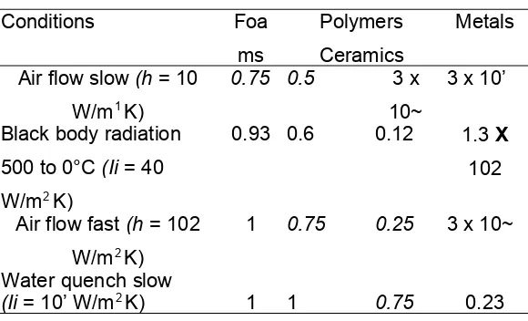
where t is a typical dimension of the sample in the direction of heat flow; the quantity (h/A is usually called the Biot modulus. Table 4.2 gives typical values of A,
for each class, using a section size of 10 mm~
The equation defining the thermal shock resistance, AT, now becomes
-BLiT--~-’
— aE (4.24)
where B = C/A. The contours on the diagram are of BAT. The table shows that,
for rapid quenching, A is unity for all materials except the high conductivity
Water quench fast
(h = 10~ W/m’ K) 1 1 1 ~0.S
shock resistance is simply read from the contours, with appropriate correction for the
constraint (the factor C). For slower quenches, t~ T is larger by the factor 1/A, read from the table.
The Strength — Temperature Chart (Chart 13, Fig. 4.14)
As the temperature of a solid is raised, the amplitude of the thermal vibration of
their atoms increases and the solid expands. Both the expansion and the vibrational
energy make plastic flow easier. The strength of solids falls, very slowly at first and
then more rapidly, as the temperature increases. Chart 13 (Fig. 4.14) captures some
of this information. It shows the yield strength (at a “normal” test strain rate of 104/s)
plotted against temperature. The near horizontal part of each lozenge shows the
strength in the regime in which temperature has little effect; the downward sloping
part shows the more precipitate drop.
There are much better ways of describing high-temperature strength than this, but
they are much more complicated. The chart gives a bird’s-eye view of the regimes of
stress and temperature in which each material class, and material, is usable. Note
that even the best polymers have very little strength above 200°C; metals become
very soft by 800°C; and only ceramics offer strength above 1000°C.
The Modulus — Relative Cost Chart (Chart 14, Fig. 4.15)
Properties like modulus, ‘strength or conductivity do not change with time. Cost is
bothersome because it does. Supply, scarcity, speculation and inflation contribute to
the considerable fluctuations in the cost per kilogram of a commodity like copper.
Data for cost per kg are tabulated for some materials in daily papers and trade
journals; those for others are harder to come by. To remove the influence of inflation
and the units Of the currency in which cost is measured, we define a relative cost
CR:
— Cost per kg of the material
At the time of writing, steel reinforcing rod costs about £0.2/kg (US$ 0.4/kg).
Chart 14 (Fig. 4.15) shows the modulus E plotted against relative cost per unit volume CRP, where p is the density. Cheap stiff materials lie fowards the top left. Expensive compliant materials lie towards the bottom right.
The Strength — Relative Cost Chart (Chart 15, Fig. 4.16)
Cheap strong materials are selected using Chart 15 (Fig. 4.16). It shows strength,
defined as before, plotted against relative cost, defined above. The qualifications on
the definition of strength, given earlier, apply here also.
It must be emphasised that the data plotted here and on Chart 14 are less reliable than those of previous charts, and subject to unpredictable change.
Despite this dire warning, the two charts are genuinely useful. They allow
selection of materials, using the criterion of “function per unit cost”. An
example is given in Chapter 6, Section 6.19.
52 Materials Selection in Mechanical Design
The Wear Rate — Bearing Pressure Chart (Chart 16, Fig. 4.17)
Wear presents a new class of problem: it is not aproperty of one material, but that of
one material sliding on another, with — if lubricated — a third in between. The
number of combinations is far too large to hope to deal with it neatly. The best we
can do is to display the range of wear rates expected under sbme standard condition
— dry sliding on a steel counterface, for instance.
The wear rate is defined as
— volume of material removed
distance of sliding
It has units of m2. At low bearing pressures P (the force pressing the two
W=KAAP
where KA is a constant, the Archard constant, with units of (MPa) ~. But as a characteristic maximum bearing pressure Pmax is approached, KA rises steeply. Chart 16 (Fig. 4.17) shows the constant KA plotted against bearing pressure P. Each lozenge shows the constant value of KA at low P, and the steep rise as Pm~ is approached. Materials cannot be used above Pm~. An example of the use of the chart is given in Section 6.20.
The Environmental Attack Chart (Chart 17, Fig. 4.18)
Corrosion, like wear, depends both on the material and on its environment. It cannot
be quantified in any general way. Data books and bases generally rank the
resistance of a material to attack in a given environment according to a scale such
as “A” (wonderful) to “D” (awful). This information is shown, for six environments in
Chart 17 (Fig. 4.18). Its usefulness is very limited; at best it gives warning of a
potential environmental hazard associated with the use of a given material.
4.4 Summary and Conclusions
The engineering properties of materials are usefully displayed as material selection
charts. The charts summarise the information in a compact, easily accessible way;
and they show the range of any given property accessible to the designer and
indentify the material class associated with segments of that range. By choosing the
axes in a sensible way, more information can be displayed: a chart of modulus E
against density p reveals the longitudinal wave velocity (EIp) ‘~ a plot of fracture toughness Kfr against modulus E shows the fracture surface energy Gk; a diagram of thermal conductivity A against diffusivity, a, also gives the volume specific heat
pC~ expansion, a, against normalised strength, c,/E, gives thermal shock resistance
AT.
The most striking feature of the charts is the way in which members of a material
with metals (as an example), they occupy a field which is distinct from that of
polymers, or that of ceramics, or that of composites. The same is true of strength,
toughness, thermal conductivity and the rest:
the fields sometimes overlap, but they always have a characteristic place within
the whole picture.
The position of the fields and their relationship can be understood in simple physical
terms:
the nature of the bonding, the packing density, the lattice resistance and the
vibrational modes of the structure (themselves a function of bonding and
packing), and so forth. It may seem odd that so little mention has been made
of microstructure in determining properties. But the charts clearly show that
the first-order difference between the properties of materials has its origins in
the mass of the atoms, the nature of the interatomic forces and the geometry
of
packing. Alloying, heat treatment and mechanical working all influence
microstructure, and through this, properties, giving the elongated bubbles shown on
many of the charts; but the magnitude of their effect is less, by factors of 10, than
that of bonding and structure.
The charts have numerous applications. One is the checking and validation of data
(Chapter 11); here use is made both of ~the range covered by the envelope of
material properties, and of the numerous relations between material properties (like
E~2 = 100 kT~,), described in Section 4.3. Another concerns the development of, and identification of uses for, new materials (Chapter 14); materials which fill gaps in
one or more of the charts generally offer some improved design potential. But most
important of all, the charts form the basis of a procedure for materials selection. That
is developed in the next four chapters.
4.5 Further Reading
The best book on the physical origins of the mechanical properties of
materials remains that by Cottrell (1964). There is no single source of data
shown on the charts. The rest comes from original papers, reports and
suppliers’ data sheets.
Material Properties: General
Cottrell, A. H. (1964) Mechanical Properties of Matter. Wiley, NY, USA. Tabor, D. (1978) Properties of Matter. Penguin Books, London, UK.
Handbooks of Material Properties
American Institute of Physics Handbook (1972~ 3rd edition. McGraw Hill, New York. USA.
ASM Metals Handbook (1973) 8th edition. American Society for Metals, Columbus, Ohio, USA.
Handbook of Chemistry and Physics (1971) 52nd edition. The Chemical Rubber Co., Cleveland, Ohio, USA.
Landolt-Borastein Tab/es (1966) Springer, Berlin, Germany.
Materials Selector (1992) Material Engineering. Panton Publishing, Cleveland, Ohio, USA.
Smithells, C. J. (1984) Metals Reference Book, 6th edition. Butterworths, London, UK.
Handbook of Plastics and Elastomers (1975) Editor C. A. Harper. McGraw Hill, New York. USA.
Bhowmick, A. K. and Stephens, H. L. (1988) Handbook of Elaslomers. Marcel Dekker, NY, USA.
Handbook of Physical Constants (1966) Memoir 97. Editor S. P. Clarke, mr. The Geological Society of America, New York, USA.
Elsevier Materials Selector (1991) Elsevier, Amsterdam.
Morrell, R. (1985, 1987) Handbook of Properties of Technical and Engineering Ceramics Paris! and 11. National Physical Laboratory, Her Majesty’s Stationery Office, London, UK.
Dinwoodie, J. M. (1981) Timber, Its Nature and Behaviour. Van Nostrand-Reinhold, Wokingham, UK.