Ch14-Multicriteria Decision Making

Introduction to Management Science

(8th Edition, Bernard W. Taylor III)

Chapter 14

Goal Programming

Graphical Interpretation of Goal Programming

Computer Solution of Goal Programming Problems with

Chapter Topics

Computer Solution of Goal Programming Problems with QM for Windows and Excel

Study of problems with several criteria, multiple criteria,

instead of a single objective when making a decision.

Two techniques discussed: goal programming, and the

Overview

Two techniques discussed: goal programming, and the

analytical hierarchy process.

Goal programming is a variation of linear programming considering more than one objective (goals)

in the objective function.

Beaver Creek Pottery Company Example:

Maximize Z = $40x₁ + 50x₂

Goal Programming

Model Formulation (1 of 2)

subject to:

1x₁ + 2x₂  40 hours of labor 4x₂ + 3x₂  120 pounds of clay x₁, x₂  0

Adding objectives (goals) in order of importance, the company:

Does not want to use fewer than 40 hours of labor per

Goal Programming

Model Formulation (2 of 2)

Does not want to use fewer than 40 hours of labor per day.

Would like to achieve a satisfactory profit level of $1,600 per day.

Prefers not to keep more than 120 pounds of clay on hand each day.

hand each day.

All goal constraints are equalities that include deviational variables d- _{and d}+_.

A positive deviational variable (d+_{) is the amount by which a}

Goal Programming

Goal Constraint Requirements

A positive deviational variable (d+_{) is the amount by which a}

goal level is exceeded.

A negative deviation variable (d-_{) is the amount by which a}

goal level is underachieved.

At least one or both deviational variables in a goal constraint must equal zero.

constraint must equal zero.

Labor goals constraint (1, less than 40 hours labor; 4, minimum overtime):

Goal Programming

Goal Constraints and Objective Function (1 of 2)

Minimize P₁d₁-_{, P}

4d1+

Add profit goal constraint (2, achieve profit of $1,600):

Minimize P₁d₁-_{, P}

2d2-, P4d1+

Add material goal constraint (3, avoid keeping more than 120 pounds of clay on hand):

120 pounds of clay on hand):

Minimize P₁d₁-_{, P}

Complete Goal Programming Model:

Minimize P₁d₁-_{, P}

2d2-, P3d3+, P4d1+

Goal Programming

Goal Constraints and Objective Function (2 of 2)

subject to:

x₁ + 2x₂ + d₁- _{- d}

1+ = 40

40x₁ + 50 x₂ + d₂ - _{- d}

2 + = 1,600

4x₁ + 3x₂ + d₃ - _{- d}

3 + = 120

x₁, x₂, d₁ -_{, d}

Changing fourth-priority goal limits overtime to 10 hours instead of minimizing overtime:

d - _{+ d} - _{- d} + _{= 10}

Goal Programming

Alternative Forms of Goal Constraints (1 of 2)

d₁- _{+ d}

4 - - d4+ = 10

minimize P₁d₁ -_{, P}

2d2 -, P3d3 +, P4d4 +

Addition of a fifth-priority goal- “important to achieve the goal for mugs”:

x₁ + d₅ - _{= 30 bowls}

x₂ + d₆ - _{= 20 mugs}

minimize P₁d₁ -_{, P}

-Goal Programming

Alternative Forms of Goal Constraints (2 of 2)

Complete Model with New Goals:

Minimize P₁d₁-_{, P}

2d2-, P3d3-, P4d4-, 4P5d5-, 5P5d6

-subject to:

x₁ + 2x₂ + d₁- _{- d}

1+ = 40

40x₁ + 50x₂ + d₂- _{- d}

2+ = 1,600

4x₁ + 3x₂ + d₃- _{- d}

3+ = 120

d₁+ _{+ d}

4- - d4+ = 10

x₁ + d₅- _{= 30}

x + d1 5- _{= 20}

x₂ + d₆- _{= 20}

x₁, x₂, d₁-_{, d}

Goal Programming

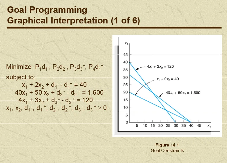
Graphical Interpretation (1 of 6)

Minimize P₁d₁-_{, P}

2d2-, P3d3+, P4d1+

subject to:

x₁ + 2x₂ + d₁- _{- d}

1+ = 40

40x₁ + 50 x₂ + d₂ - _{- d}

2 + = 1,600

4x₁ + 3x₂ + d₃ - _{- d}

3 + = 120

x₁, x₂, d₁ -_{, d}

1 +, d2 -, d2 +, d3 -, d3 +  0

Figure 14.1

Goal Programming

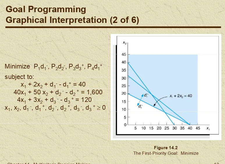
Graphical Interpretation (2 of 6)

Minimize P₁d₁-_{, P}

2d2-, P3d3+, P4d1+

subject to:

x₁ + 2x₂ + d₁- _{- d}

1+ = 40

40x₁ + 50 x₂ + d₂ - _{- d}

2 + = 1,600

4x₁ + 3x₂ + d₃ - _{- d}

3 + = 120

x₁, x₂, d₁ -_{, d}

1 +, d2 -, d2 +, d3 -, d3 +  0

Figure 14.2

Goal Programming

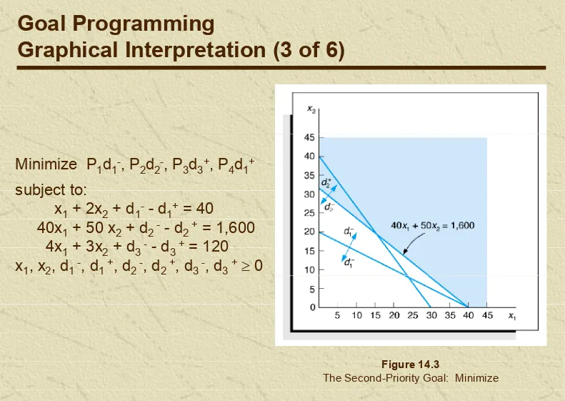
Graphical Interpretation (3 of 6)

Minimize P₁d₁-_{, P}

2d2-, P3d3+, P4d1+

subject to:

x₁ + 2x₂ + d₁- _{- d}

1+ = 40

40x₁ + 50 x₂ + d₂ - _{- d}

2 + = 1,600

4x₁ + 3x₂ + d₃ - _{- d}

3 + = 120

x₁, x₂, d₁ -_{, d}

1 +, d2 -, d2 +, d3 -, d3 +  0

Figure 14.3

Goal Programming

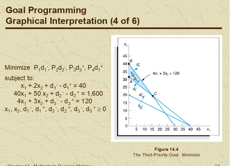
Graphical Interpretation (4 of 6)

Minimize P₁d₁-_{, P}

2d2-, P3d3+, P4d1+

subject to:

x₁ + 2x₂ + d₁- _{- d}

1+ = 40

40x₁ + 50 x₂ + d₂ - _{- d}

2 + = 1,600

4x₁ + 3x₂ + d₃ - _{- d}

3 + = 120

x₁, x₂, d₁ -_{, d}

1 +, d2 -, d2 +, d3 -, d3 +  0

Figure 14.4

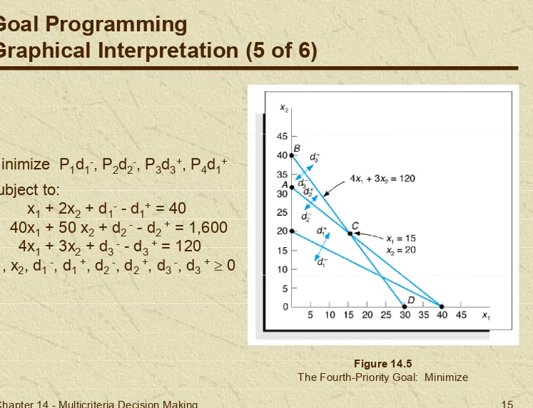
Goal Programming

Graphical Interpretation (5 of 6)

Minimize P₁d₁-_{, P}

2d2-, P3d3+, P4d1+

subject to:

x₁ + 2x₂ + d₁- _{- d}

1+ = 40

40x₁ + 50 x₂ + d₂ - _{- d}

2 + = 1,600

4x₁ + 3x₂ + d₃ - _{- d}

3 + = 120

x₁, x₂, d₁ -_{, d}

1 +, d2 -, d2 +, d3 -, d3 +  0

Figure 14.5

Goal programming solutions do not always achieve all goals and they are not optimal, they achieve the best or most

satisfactory solution possible.

Goal Programming

Graphical Interpretation (6 of 6)

satisfactory solution possible.

Minimize P₁d₁-_{, P}

2d2-, P3d3+, P4d1+

subject to:

x + 2x + d - _{- d} + _{= 40}

Goal Programming

Computer Solution Using QM for Windows (1 of 3)

x₁ + 2x₂ + d₁- _{- d}

1+ = 40

40x₁ + 50 x₂ + d₂ - _{- d}

2 + = 1,600

4x₁ + 3x₂ + d₃ - _{- d}

3 + = 120

x₁, x₂, d₁ -_{, d}

1 +, d2 -, d2 +, d3 -, d3 +  0

Goal Programming

Computer Solution Using QM for Windows (2 of 3)

Goal Programming

Computer Solution Using QM for Windows (3 of 3)

Goal Programming

Computer Solution Using Excel (1 of 3)

Goal Programming

Computer Solution Using Excel (2 of 3)

Goal Programming

Computer Solution Using Excel (3 of 3)

Minimize P₁d₁-_{, P}

2d2-, P3d3-, P4d4-, 4P5d5-, 5P5d6

-subject to:

Goal Programming

Solution for Altered Problem Using Excel (1 of 6)

subject to:

x₁ + 2x₂ + d₁- _{- d}

1+ = 40

40x₁ + 50x₂ + d₂- _{- d}

2+ = 1,600

4x₁ + 3x₂ + d₃- _{- d}

3+ = 120

d₁+ _{+ d}

4- - d4+ = 10

x₁ + d₅- _{= 30}

x₂ + d₆- _{= 20}

x , x , d2 6 -_{, d} +_{, d} -_{, d} +_{, d} -_{, d} +, _d -_{, d} +_{, d} -_{, d} -  ₀

x₁, x₂, d₁-_{, d}

Goal Programming

Solution for Altered Problem Using Excel (2 of 6)

Goal Programming

Solution for Altered Problem Using Excel (3 of 6)

Goal Programming

Solution for Altered Problem Using Excel (4 of 6)

Goal Programming

Solution for Altered Problem Using Excel (5 of 6)

Goal Programming

Solution for Altered Problem Using Excel (6 of 6)

AHP is a method for ranking several decision alternatives and selecting the best one when the decision maker has multiple objectives, or criteria, on which to base the

Analytical Hierarchy Process

Overview

multiple objectives, or criteria, on which to base the decision.

The decision maker makes a decision based on how the alternatives compare according to several criteria.

The decision maker will select the alternative that best meets his or her decision criteria.

Southcorp Development Company shopping mall site selection.

Three potential sites:

Analytical Hierarchy Process

Example Problem Statement

Three potential sites:

Atlanta

Birmingham

Charlotte.

Criteria for site comparisons:

Customer market base.

Income level

Top of the hierarchy: the objective (select the best site).

Second level: how the four criteria contribute to the objective.

Analytical Hierarchy Process

Hierarchy Structure

objective.

Mathematically determine preferences for each site for each criteria.

Mathematically determine preferences for criteria (rank

Analytical Hierarchy Process

General Mathematical Process

Mathematically determine preferences for criteria (rank order of importance).

Combine these two sets of preferences to mathematically derive a score for each site.

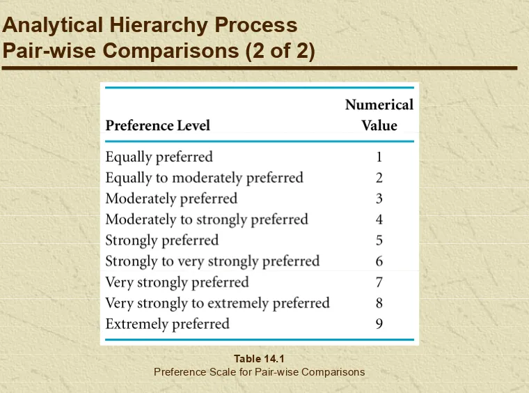
In a pair-wise comparison, two alternatives are compared according to a criterion and one is preferred.

A preference scale assigns numerical values to different

Analytical Hierarchy Process

Pair-wise Comparisons

Analytical Hierarchy Process

Pair-wise Comparisons (2 of 2)

Table 14.1

Analytical Hierarchy Process

Pair-wise Comparison Matrix

A pair-wise comparison matrix summarizes the pair-wise comparisons for a criteria.

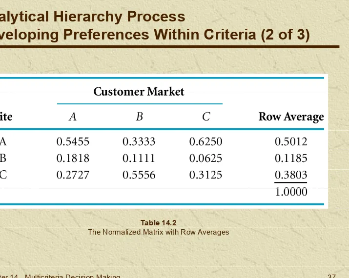
Analytical Hierarchy Process

Developing Preferences Within Criteria (1 of 3)

In synthetization, decision alternatives are prioritized with each criterion and then normalized:

Analytical Hierarchy Process

Developing Preferences Within Criteria (2 of 3)

Table 14.2

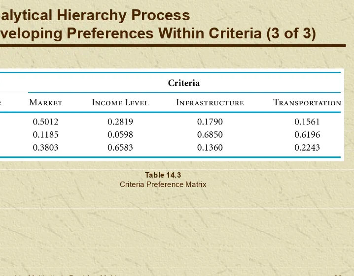
Analytical Hierarchy Process

Developing Preferences Within Criteria (3 of 3)

Table 14.3

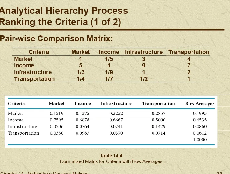
Criteria Market Income Infrastructure Transportation

Market 1 1/5 3 4

Analytical Hierarchy Process

Ranking the Criteria (1 of 2)

Pair-wise Comparison Matrix:

Market



Analytical Hierarchy Process

Ranking the Criteria (2 of 2)

Overall Score:

Site A score = .1993(.5012) + .6535(.2819) + .0860(.1790) + .0612(.1561) = .3091

Analytical Hierarchy Process

Developing an Overall Ranking

.0860(.1790) + .0612(.1561) = .3091

Site B score = .1993(.1185) + .6535(.0598) + .0860(.6850) + .0612(.6196) = .1595

Site C score = .1993(.3803) + .6535(.6583) + .0860(.1360) + .0612(.2243) = .5314

Overall Ranking:

Site Score Charlotte

Atlanta Birmingham

Analytical Hierarchy Process

Summary of Mathematical Steps

Develop a pair-wise comparison matrix for each decision alternative for each criteria.

Synthetization Synthetization

Sum the values of each column of the pair-wise comparison matrices.

Divide each value in each column by the corresponding column sum.

Average the values in each row of the normalized matrices. Combine the vectors of preferences for each criterion.

Develop a pair-wise comparison matrix for the criteria. Develop a pair-wise comparison matrix for the criteria. Compute the normalized matrix.

Develop the preference vector.

Goal Programming

Excel Spreadsheets (1 of 4)

Goal Programming

Goal Programming

Excel Spreadsheets (3 of 4)

Goal Programming

Excel Spreadsheets (4 of 4)

Each decision alternative graded in terms of how well it satisfies the criterion according to following formula:

S = g w

Scoring Model

Overview

S_i = g_ijw_j

where:

w_j = a weight between 0 and 1.00 assigned to criteria j; 1.00 important, 0 unimportant; sum of total weights

equals one.

g = a grade between 0 and 100 indicating how well g_ij = a grade between 0 and 100 indicating how well alternative i satisfies criteria j; 100 indicates high

Mall selection with four alternatives and five criteria:

Scoring Model

Excel Solution

Goal Programming Example Problem

Problem Statement

Public relations firm survey interviewer staffing requirements determination.

One person can conduct 80 telephone interviews or 40 personal One person can conduct 80 telephone interviews or 40 personal interviews per day.

$50/ day for telephone interviewer; $70 for personal interviewer.

Goals (in priority order):

At least 3,000 total interviews.

Interviewer conducts only one type of interview each day. Maintain daily budget of $2,500.

daily budget of $2,500.

At least 1,000 interviews should be by telephone.

Formulate a goal programming model to determine number of

Step 1: Model Formulation:

Minimize P₁d₁-_{, P}

2d2-, P3d3

-Goal Programming Example Problem

Solution (1 of 2)

subject to:

80x₁ + 40x₂ + d₁- _{- d}

1+ = 3,000 interviews

50x₁ + 70x₂ + d₂- _{- d}

2 + = $2,500 budget

80x₁ + d₃- _{- d}

3 + = 1,000 telephone interviews

where:

Goal Programming Example Problem

Solution (2 of 2)

Purchasing decision, three model alternatives, three decision criteria.

Pair-wise comparison matrices:

Analytical Hierarchy Process Example Problem

Problem Statement

Pair-wise comparison matrices:

Step 1: Develop normalized matrices and preference

vectors for all the pair-wise comparison matrices for criteria.

Analytical Hierarchy Process Example Problem

Problem Solution (1 of 4)

Price

Bike X Y Z Row Averages

X

Bike X Y Z Row Averages

Step 1 continued: Develop normalized matrices and

preference vectors for all the pair-wise comparison matrices for criteria.

Analytical Hierarchy Process Example Problem

Problem Solution (2 of 4)

Weight/Durability

Bike X Y Z Row Averages

X

Step 2: Rank the criteria.

Criteria Price Gears Weight Row Averages

Analytical Hierarchy Process Example Problem

Problem Solution (3 of 4)

Step 3: Develop an overall ranking.

Bike X 0.6667 0.0853 0.4429 0.6479

Analytical Hierarchy Process Example Problem

Problem Solution (4 of 4)

Bike X Bike Y Bike Z

Bike X score = .6667(.6479) + .0853(.2299) + .4429(.1222) = .5057 Bike Y score = .2222(.6479) + .2132(.2299) + .1698(.1222) = .2138



Bike Y score = .2222(.6479) + .2132(.2299) + .1698(.1222) = .2138 Bike Z score = .1111(.6479) + .7014(.2299) + .3873(.1222) = .2806