3D Indoor Building Environment Reconstruction using Least Square Adjustment, Polynomial
Kernel, Interval Analysis and Homotopy Continuation
Ali Jamali1, François Anton2, Alias Abdul Rahman1 and Darka M ioc2
1) Universiti Teknologi M alaysia (UTM ) Faculty of Geoinformation and Real Estate
[email protected], [email protected]
2) Technical University of Denmark, Denmark National Space Institute,
[email protected], [email protected]
KEY WORDS : Indoor surveying, least square adjustment, interval analysis, laser scanning, calibration, homotopy continuation ABS TRACT:
Nowadays, municipalities intend to have 3D city models for facility management, disaster management and architectural planning. Indoor models can be reconstructed from construction plans but sometimes, they are not available or very often, they differ f rom
‘as-built’ plans. In this case, the buildings and their rooms must be surveyed. One of the most utilized methods of indoor surveying is laser scanning. The laser scanning method allows taking accurate and detailed measurements. However, Terrestrial Laser Scanner is costly and time consuming. In this paper, several techniques for indoor 3D building data acquisition have been investigated. For reducing the time and cost of indoor building data acquisition process, the Trimble LaserAce 1000 range finder is us ed. The proposed approache use relatively cheap equipment: a light Laser Rangefinder which appear to be feasible, but it needs to be tested to see if the observation accuracy is sufficient for the 3D building modelling. The accuracy of the rangefinder is evaluated and a simple spatial model is reconstructed from real data. This technique is rapid (it requires a shorter time as compared to others), but the results show inconsistencies in horizontal angles for short distances in indoor environments. The range finder horizontal angle sensor was calibrated using a least square adjustment algorithm, a polynomial kernel, interval analysis and homotopy continuation.
1.
Introduction
The automatic reconstruction of urban 3D models has been a research area of photogrammetry for the past two decades (Haala and Kada, 2010). According to Habib et al. (2010), digital 3D modelling of complex buildings has been a challenge until now with photogrammetry technology. This leads towards semi-automated construction of complex 3D building models. Difficulties of interpretation of photogrammetric images for 3D city modelling, especially for complex buildings, motivated increasing demands for 3D point cloud technologies such as LiDAR (light detection and ranging), which can facilitate automated 3D building models.
According to Surmann et al. (2003), rapid characterization and quantification of complex environments with increasing demands has created a challenge for 3D data analysis. This crucial demand comes from different fields such as industrial automation, architecture, agriculture, construction and mine and tunnel maintenance. Precise 3D data is needed for facility management, factory design and regional and urban planning. Considering all the issues affecting fully automated construction of complex 3D building models, 3D indoor modelling is another aspect in the field of 3D city modelling which can make the current situation more
complex. According to Deak et al. (2012), indoor location determination has become a crucial aspect in many different applications but unfortunately, a lack of standard is one of the challenges and there are more challenges encountered in this field. According to Donath and Thurow (2007), considering many fields of applications for buildin g surveying and resulting different demands, representation of the building geometry is the most crucial aspect of a building survey. Due to the complexity of indoor environment, this field needs to be more researched.
technology can collect more than 500,000 points in a second with an accuracy of ±6 mm (Dongzhen et al., 2009).
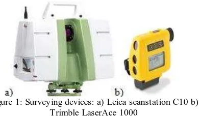
In this research, we provide a comparative analysis of 3D reconstruction and indoor survey of a building done using the Leica scanstation C10 and the Trimble LaserAce 1000 rangefinder (see Figure 1). The Trimble LaserAce 1000 has been used for outdoor mapping and measurements, such as forestry measurement and GIS mapping (Jamali et al., 2013). A rangefinder can be considered as a basic mobile Total Station with limited functionality and low accuracy. The Trimble LaserAce 1000 is a three-dimensional laser rangefinder with point and shoot workflow. This rangefinder includes a pulsed laser distance meter and a compass, which can measure distance, horizontal angle and vertical angle up to 150 meter without a target and up to 600 meter with a reflective foil target. In this research, we propose this device for indoor mapping and try to validate this technique in an indoor environment. Trimble LaserAce 1000 will decrease time and cost of surveying process (Jamali et al. 2015).
Figure 1: Surveying devices: a) Leica scanstation C10 b) Trimble LaserAce 1000
Following this introduction, in Section 2, the requirements of indoor building surveying are discussed. In Section 3, the range finder is calibrated using a least square adjustment algorithm. In section 4, the rangefinder is calibrated using a polynomial kernel. In Section 5, the range finder is calibrated using interval analysis and homotopy continuation in order to control the uncertainty of the calibration and of the reconstruction of the building. Section 6 presents conclusions and future research.
2. REQUIREMENTS OF AN INDOOR
BUILDING S URVEYING METHOD
In this research, the surveyor according to his experience and knowledge defined several requirements for indoor building surveying as follows:
i. Number of control points and their positions
To get better results with less shape deformation (e.g. intersection and gap between two rooms due to low accuracy of Trimble LaserAce 1000), for each door, there should be a control point inside the corridor. For example, if a room has two doors, there should be two control points in the corridor to access that certain room by its two doors (see Figure 2).
Figure 2: Position of control points by Trimble LaserAce 1000
To avoid narrow and wide angle propagation which will lead to shape deformation, Trimble LaserAce 1000 needs to be stationed in the center of each room. In reality, there will be some furniture in rooms which avoids putting Trimble LaserAce 1000 in the center of a room. Thus, for a fully furnished room, there should be at least two control points.
i. Number of repetitions of measurements
Based on the surveyor’s skills, for a certain distance and
angle measurement, there should be at least three observations. Trimble LaserAce 1000 shows inconsistency in horizontal angle in an indoor building environment. By increasing number of repetitions for a measurement, the probability of a mistake or blunder occurring will be decreased. In this paper, we use least squares adjustment as a statistical method and interval analysis and homotopy continuation as mathematical methods to calibrate our low accuracy surveying equipment in an indoor building environment. Thus, a higher number of measurements will led to a more accurate average using least square adjustment and more accurate measurement intervals using interval analysis and homotopy continuation.
ii. Time
Figure 3: Time of data collection and 3D building modeling
i. Cost
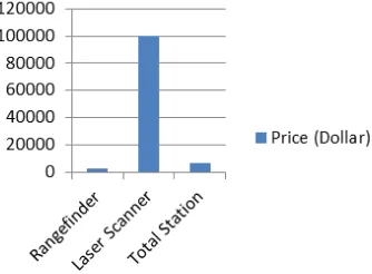
The cost of the rangefinder is very low compared to the other devices (laser scanner and Total Station) used in this research (See Figure 4).
Figure 4: Equipment comparison based on the cost.
i. Data storage
Data storage for a floor collected by Trimble LaserAce 1000 with twelve rooms and one corridor is around 10 Kilo Bytes (KB) in Object model (.obj) data format, 14 KB in Geogebra data format without control points and 38 KB with control points. Data collected by Leica scanstation C10 occupies 4.18 Giga Bytes (GB). Data collected using Leica scanstation C10 contains unnecessary details such as furniture and installations. Data storage, rendering and modeling need to be considered as important factors in most of applications. Navigation through a building (Yuan and Schneider 2010; Li and He 2008; Goetz and Zipf 2011) is possible by nodes and lines (paths or edges) and 3D building models allow a better understanding of the real world environment.
3. RANGEFINDER CALIBRATION
Coordinates measured by rangefinder are not as precise as laser scanner or total station measurements. As seen in Figures 5 and 6, results of Trimble LaserAce 1000 shows deformation of building geometry.
Figure 5: Floor plan by Trimble LaserAce 1000.
Figure 6: 3D building modelling of room 9 by Trimble LaserAce 1000 where dash lines represent measured data
from Trimble LaserAce 1000 and solid lines represent extruded floor plan.
Figure 7 shows a 3D point cloud collected by Leica scanstation C10.
Figure 7: point cloud data collected by Leica scanstation C10
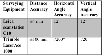
According to device specifications, the accuracies of the Leica scanstation C10, Trimble LaserAce 1000 are as shown in Table 1.
S urveying
The 3D building measured by the Trimble LaserAce 1000 can be calibrated and reconstructed from the Leica scanstation C10 based on the least square adjustment algorithm, in the form of absolute orientation. Least square adjustment is a well-known algorithm in surveying engineering which is used widely by engineers to get the best solution in the sense of the minimization of the sum of the squares of the residuals, which is obtained as in the following normal equations, which express that the total differential of the sum of squares of residuals is zero. Least square adjustment for a linear system is shown in Equation (1).
X = (AT WA)-1AT W L
X= N-1 AT W L (1)
Where L = observations X = unknowns
A = coefficient of unknowns
W=observation’s weight
N = (AT W A)
Considering two points, Pa= (XA, YA, ZA) from the Leica C10 and Pc= (XC, YC, ZC) from the Trimble LaserAce 1000, the absolute orientation problem can be defined as the transformation between two coordinates systems (Leica C10 and Trimble LaserAce 1000). The relationship between measuring devices can be solved by using absolute orientation. Absolute orientation can be found by a set of conjugate pairs: {(Pc,l, Pa,l), (Pc,2 Pa,2), ... , (Pc,n, Pa,n)}. For a pair of common points in both (camera coordinates and absolute coordinates) systems; rotation, scale and translation
components can be calculated by Equations 2 to 4, where the matrix R with coefficients RXX, RXY, RXZ, RYX, RYY, RYZ, RZX, RZY and RZZ, is the matrix of a linear transformation combining a 3D rotation (that can be decomposed into the combinations of 3 rotations along the x, y and z axes) and a scaling, and its determinant is the scaling parameter (since the determinant of a rotation matrix must equal 1).
XA=RXX XC + RXY YC + RXZ ZC + TX (2) YA=RYX XC + RYY YC + RYZ ZC + TY (3) ZA=RZX XC + RZY YC + RZZ ZC + TZ (4)
Twelve unknown parameters, including nine linear transformation (combined rotation and scaling) parameters and three translations components need to be solved. Each conjugate pair yields three equations. The minimum number of required points to solve for the absolute orientation is thus four common points. Practically, to get better results with higher accuracy, a higher number of points need to be used. The coordinates of the points measured by the rangefinder can be adjusted, or their maximum error can be minimized, by adjusting the coefficients of the rotation matrix R and the translation vector (see adjustment results in Table 2). Room number nine has been selected by the researcher to calculat e its absolute orientation parameters.
Table 2: Coefficient of unknowns including rotation, scale and translation parameters (matrix A).
R X
Table 3: LaserAce 1000 calibration based on the least square adjustment (Absolute orientation). Point
Number
X LaserAce Y LaserAce Z LaserAce X Leica C10 Y Leica C10 Z Leica C10
1 10.394 3.7777 1.1067 10.424 3.725 1.105
2 2.0673 2.3577 1.1122 2.131 2.249 1.109
3 2.0098 3.2969 1.1098 1.956 3.355 1.109
4 1.4469 3.1347 1.1094 1.396 3.257 1.116
5 0.0059 10.678 1.11 0.047 10.605 1.108
6 8.8322 12.192 1.1128 8.803 12.246 1.115
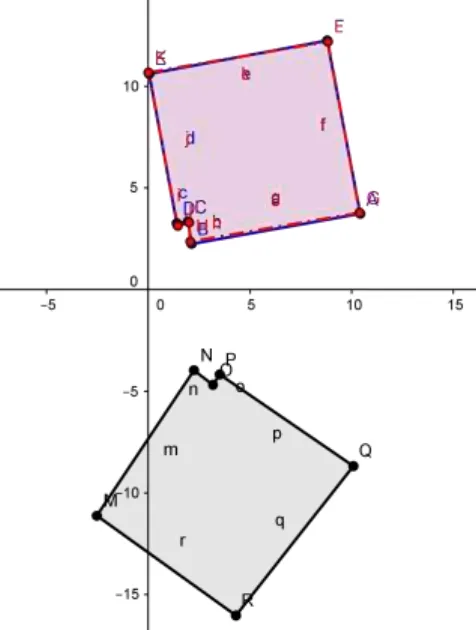
Considering the Leica C10 data as absolute coordinates, differences between two coordinates can be referred as the Trimble LaserAce 1000 accuracy. The model calibrated and reconstructed using the Leica C10 is shown in Figure. 8. M odel in black lines represents model reconstructed from
raw data of Trimble LaserAce 1000 and model in blue lines represents model reconstructed from Leica C10. Calibrated model of Trimble LaserAce 1000 based on the least square adjustment algorithm from Leica C10 data can be seen as red dash line model (see Figure 8).
Figure 8: M odel calibrated and reconstructed based on the least square adjustment; rangefinder (red dash lines), total station (blue lines) and non-calibrated rangefinder (black lines).
4. POLYNOMIAL KERNEL
In this section, polynomial kernel as a parametric non-linear method is used to calibrate Trimble LaserAce 1000 horizontal angle. In kernel methods, data is embedded into a vector space and then linear and non-linear relations between
data will be investigated. Basically, kernels are functions that return inner products between of the images of data points in vector space. Each kernel k(x,z) has an associated feature mapping � which takes input x∈X (input space) and maps it to F (feature space). Kernel k(x,z), takes two inputs and gives their similarity in F space (� = � → � � =
F needs to be a vector space with a dot product to define it, also called a Hilbert space (Browder and Petryshyn, 1967; Akhiezer and Glazman, 2013). For k to be a kernel function, a Hilbert space F must exist and k must define a dot p roduct and be positive definite (∫ �∫ � � � �, � � > 0 .
There are several kernel function including linear kernel (� �,� = ��� , quadratic kernel (k x,z = x�z 2 , polynomial kernel (k x,z = x�z� and Radial Basis Function (RBF) kernel (� �,� = ��[−�‖� − �‖2] .
Table 4: Calibration of room 1 rangefinder horizontal angle measurements using total station horizontal angle measurements by
Table 5: Calibration of room 10 rangefinder horizontal angle measurements using total station horizontal angle measurements by polynomial kernel calculated from room 1.
Point Horizontal angle
5. INTERVAL ANALYS IS AND HOMOTOPY CONTINUATION Interval analysis is a well-known method for computing bounds of a function, being given bounds on the variables of that function (E. Ramon M oore and Cloud, 2009). The basic mathematical object in interval analysis is the interval instead of the variable. The operators need to be redefined to operate on intervals instead of real variables. This leads to an interval arithmetic. In the same way, most usual mathematical functions are redefined by an interval equivalent. Interval analysis allows one to certify computations on intervals by providing bounds on the results. The uncertainty of each measure can be represented using an interval defined either by a lower bound and a higher bound or a midpoint value and a radius.
In this paper, we use interval analysis to model the uncertainty of each measurement of horizontal angle and horizontal distance done by the range finder. We represent the geometric loci corresponding to each surveyed point as functions of the bounds of each measurement. Thus, for distances observed from a position of the range finder, we represent the possible position of the surveyed point by two concentric circles centered on the position of the range finder and of radii the measured distance plus and minus the
uncertainty on the distance respectively (see Figure 9). For horizontal angles observed from a position of the range finder, we represent the possible position of the surveyed point by two rays emanating from the position of the range finder and whose angles with respect to a given point or the North are the measured angle plus and minus the uncertainty on the horizontal angle respectively (see Figure 9). Therefore, the surveyed point must be within a region bounded by these 4 loci: in between 2 concentric circles and 2 rays. Proceeding in the same way for each room, we get the geometric loci for each room and for the union of the surveyed rooms (see Figure 9).
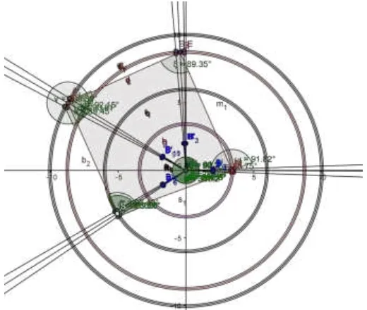
Figure 9: The geometric loci of each corner of a room as a function of all the measurements
Figure 10: Room 1 construction from original range finder measurements (red) and interval valued homotopy continuation calibration of horizontal angles measurements (blue)
A homotopy between two continuous functions f and f from a topological space X to a topological space Y is defined as
a continuous map H: X × [0, 1] → Y from the Cartesian
product of the topological space X with the unit interval [0, 1] to Y such that H(x, 0) = f0, and H(x, 1) = f1, where x ∈ X. The two functions f0 and f1 are called respectively the initial and terminal maps. The second parameter of H, also called the homotopy parameter, allows for a continuous deformation of f0 to f1 (Allgower and Georg, 1990). Two continuous functions f0 and f1 are said to be homotopic, denoted by f0 ≃ f1, if, and only if, there is a homotopy H
taking f0 to f1. Being homotopic is an equivalence relation on the set C(X, Y) of all continuous functions from X to Y.
in a digital measurement device, we can assume that all the real numbers corresponding to measurements can be obtained physically, and it is just the fixed point notation used by the digital measurement device, that limits the set of representable real numbers to a discrete subset of the set of real numbers. Thus, we can compute the calibration of the range finder as a continuous function mapping our measurements obtained using our range finder to the measurements obtained using our total station.
The results of the linear homotopy continuation are presented in Figures 10 and Tables 6-8. One can calibrate the differences of horizontal angles observed with the rangefinder to the differences of horizontal angles observed with the theodolite. One can start from any point and point and assume that the measurement of the horizontal angle of that point by the rangefinder will not be changed by the calibration process. Without loose of generality, this point can be the first observed point. Now the idea for the calibration is that we are using each one of the intervals between measurements of horizontal angles made with the rangefinder, and we calibrate the new measurements of horizontal angles made by the rangefinder in each one of these intervals as a non-linear homotopy, where the homotopy parameter is the relative position of the measured horizontal angle in between the bounds of the enclosing interval of rangefinder horizontal angles. This homotopy calibration can be visualized as the continuous deformation of each sector (defined by the rangefinder horizontal angle
intervals of room 1) of a plastic disk (corresponding to the old time theodolite graduated disk) to the corresponding sector of the total station's theodolite graduated disk. We used the intervals of total station horizontal angles of room 1 as reference intervals for all other horizontal angle measurements in rooms 1 and 10. In the remainder of the
paper, ”the homotopy parameter of a horisontal angle measurement” is equivalent to ”the relative position of the horizontal angle measurement in the corresponding
reference interval”. We fitted a polynopmial of degree 5
through the 4 points whose x-coordinates are the homotopy parameters of the horizontal angles measured by the rangefinder in room 10 and the corresponding homotopy parameters of the horizontal angles measured by the total station in room 10 and the points (0,0) and (1,1). We used this polynomial as the convex homotopy functlon that maps the uncalibrated homotopy paramter to the calibrated one.
The initial and terminal maps correspond respectively to the mappings between the uncalibrated and calibrated horizontal angles at the start point and the end point of the enclosing interval of horizontal angles measured by the range finder. We can observe that, contrary to the least squares calibration, the only limitation of this interval analysis and homotopy continuation based calibration is the precision of the fixed point arithmetic used by the computing device used for the calibration. The results shown in Table 8 proves that homotopies give the best results both in terms of RM SE and the L∞ metric.
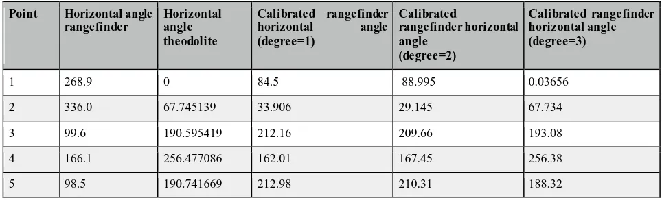
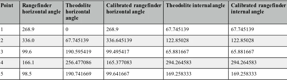
Table 6: Calibration of room 1 rangefinder horizontal angle measurements by homotopies.
Point Rangefinder
Theodolite internal angle Calibrated rangefinder internal angle
1 268.9 0 268.9 67.745139 67.745139
2 336.0 67.745139 336.645139 122.85028 122.85028
3 99.6 190.595419 99.495417 65.881667 65.881667
4 166.1 256.477086 165.377083 294.264583 294.264583
5 98.5 190.741669 99.641667 169.258333 169.258333
Table 7: Calibration of room 10 rangefinder horizontal angle measurements by homotopies
Point Horizontal angle rangefinder
Point Horizontal
The proposed research is to demonstrate the feasibility of interior surveying for full 3D building modelling.. The main objective of this research was to propose a methodology for data capturing in indoor building environment. A rangefinder was compared to a high accurate surveying device (Leica scanstation C10) using weighted least squares, polynomial kernel and a novel technique based on interval analysis and homotopy continuation. In an indoor environment, the Trimble LaserAce 1000 showed inconsistencies within the uncertainty ranges claimed by the manufacturer for short distances in the horizontal angle.
Rangefinder data was calibrated by least square adjustment (absolute orientation) which shows a maximum error of 13 centimeters and a minimum error of 6 centimeters using the Leica scanstation C10 as a benchmark. By opposition, the combined interval analysis and homotopy continuation technique calibration obtained by continuous deformation of the function mapping the rangefinder measurements to the theodolite measurements allows a much better match, whose only limitation is the fixed point arithmetic of the computing device used to perform the computation. Results from polynomial kernel are not satisfactory (see Tables 8).
7. References
Akhiezer, N. I., & Glazman, I. M . (2013). Theor y of linear oper ator s in Hilber t space. Courier Corporation.
Allgower, E. L., K. Georg, (1990). Numerical continuation methods: an introduction. Springer-Verlag New York, Inc. New York, NY, USA.
Amato, E., Antonucci, G., Belnato, B. (2003). The three dimensional laser scanner system: the new frontier for surveying, The International Archives of the Photogrammetry, Remote Sensing and Spatial Information Sciences Vol. XXXIV-5/W12, 17-22
Browder, F. E., & Petryshyn, W. V. (1967). Construction of fixed points of nonlinear mappings in Hilbert space. Jour nal of Mathematical Analysis and Applications, 20(2), 197-228.
Deak, G., Curran, K., & Condell, J. (2012). A survey of active and passive indoor localisation systems. Computer Communications, 35(16), 1939–1954.
Donath, D., & Thurow, T. (2007). Integrated architectural surveying and planning. Automation in Construction, 16(1), 19–27.
Dongzhen, J., Khoon, T., Zheng, Z., & Qi, Z. (2009). Indoor 3D M odeling and Visualization with a 3D Terrestrial Laser Scanner. 3D Geo-Information Sciences, 247–255.
Gilliéron, P. Y., & M erminod, B. (2003, October). Personal navigation system for indoor applications. In 11th IAIN wor ld congr ess (pp. 21-24).
Goetz, M ., & Zipf, A. (2011). Formal definition of a user-adaptive and length-optimal routing graph for complex indoor environments. Geo-Spatial Infor mation Science, 14(2), 119-128.
Haala, N., & Kada, M ., (2010). An update on automatic 3D building reconstruction. ISPRS Journal of Photogrammetry and Remote Sensing, 65(6), 570–580.
Li, Y., & He, Z. (2008). 3D indoor navigation: a framework of combining BIM with 3D GIS. In 44th ISOCARP congr ess.
Jamali, A., Boguslawski, P., Duncan, E. E., Gold, C. M ., & Rahman, A. A. (2013). Rapid Indoor Data Acquisition for Ladm-Based 3d Cadastre M odel. ISPRS Annals of Photogrammetry, Remote Sensing and Spatial Information Sciences, 1(1), 153-156.
Jamali, A., Abdul Rahman, A., Boguslawski, P., Kumar, P., & M . Gold, C. (2015). An automated 3D modeling of topological indoor navigation network. GeoJour nal.
Ramon M oore, R. K. E., Cloud, M . J. (2009). Introduction to interval analysis. SIAM (Society for Industrial and Applied M athematics), Philadelphia.
Surmann, H., Nüchter, A., & Hertzberg, J. (2003). An autonomous mobile robot with a 3D laser range finder for 3D exploration and digitalization of indoor environments. Robotics and Autonomous Systems, 45(3-4), 181–198.