QUALITY ASSESSMENT OF 3D RECONSTRUCTION USING FISHEYE AND
PERSPECTIVE SENSORS
C. Strecha a, R. Zoller a, S. Rutishauser a, B. Brot a, K. Schneider-Zapp a,, V.Chovancova a, M. Krull b, L. Glassey c a Pix4D SA, EPFL Innovation Park Building D, CH-1015 Lausanne – [email protected]
b 3D-Vermessungen-Krull, Hoffnungstaler Str. 39 D-58091 Hagen – [email protected] c MOSINI et CAVIEZEL SA, Rue Louis de Savoie 72, CH-1110 Morges - [email protected]
KEY WORDS:Photogrammetry, Fisheye lens, 3D-Modeling, Reconstruction, Laser Scanning, Accuracy, Point Cloud
ABSTRACT:
Recent mathematical advances, growing alongside the use of unmanned aerial vehicles, have not only overcome the restriction of roll and pitch angles during flight but also enabled us to apply non-metric cameras in photogrammetric method, providing more flexibility for sensor selection. Fisheye cameras, for example, advantageously provide images with wide coverage; however, these images are extremely distorted and their non-uniform resolutions make them more difficult to use for mapping or terrestrial 3D modelling. In this paper, we compare the usability of different camera-lens combinations, using the complete workflow implemented in Pix4Dmapper to achieve the final terrestrial reconstruction result of a well-known historical site in Switzerland: the Chillon Castle. We assess the accuracy of the outcome acquired by consumer cameras with perspective and fisheye lenses, comparing the results to a laser scanner point cloud.
1. INTRODUCTION
In recent years, more and more decent quality sensors have become available at an affordable price. In this paper, we address the question of the most suitable sensor-lens combination for terrestrial and indoor 3D modeling purposes. The goal is to identify the camera with the highest accuracy and to discuss the accuracy achieved from various data capture and processing. The use of fisheye cameras, for example, resolves the issue of limited space and restricted conditions for setting up camera stations; both problems are dominantly present in indoor and terrestrial city modelling. Fisheye lenses have a wide range of focus and their wide field of view makes it possible to capture a scene with far fewer images. This also leads to more stable and scalable bundle block adjustment on the camera’s exterior and interior orientations. These fisheye lens advantages relate to the efficiency in data capture, which today, since the processing is highly automated, contributes dominantly to the total cost of terrestrial or indoor surveying. The disadvantage of fisheye lenses is their large and very non-uniform ground sampling distance (GSD), when compared to perspective lenses. Thus, finding a good compromise between accuracy and acquisition plus processing effort is one of the major questions we address in this paper.
We began to look at fisheye lenses as a result of our previous work (C. Strecha, T. Pylvanainen, P. Fua, 2010) on large scale city modelling. It was during this work we observed that in terrestrial city modelling one needs many perspective images to reconstruct particularly narrow streets, for which fisheye lenses would help substantially to reduce the complexity and acquisition time.
2. MATERIALS AND METHODS
2.1 Software
All results were generated by Pix4Dmapper (Pix4D, 2014) version 1.2. The software is partially based on earlier published work (C. Strecha, T. Pylvanainen, P. Fua, 2010) (C. Strecha, T. Tuytelaars, L. Van Gool, 2003) (Strecha, et al., 2008) and
implements a fully automated photogrammetric workflow for indoor, terrestrial, oblique and nadir imagery. It is capable of handling images with missing or inaccurate geo-information. The approach combines the automation of computer vision techniques (C. Strecha and W. von Hansen and L. Van Gool and P. Fua and U. Thoennessen, 2008) (S. Agarwal, Y. Furukawa, N. Snavely, B. Curless, S.M. Seitz, R. Szeliski, 2012) with the photogrammetric grade accuracy.
The software supports both standard perspective camera models and equidistant fisheye camera models (Kannala, et al., 2006) (Schwalbe) (Hughes, et al., 2010). Given the world coordinates
, , in the camera centric coordinate system, the angle θ between the incident ray and the camera direction is given by:
� = arctan (√ 2+ 2) (1) point coordinate in image space. The polynomial coefficient � is redundant to the parameters , and is defined to be 1.
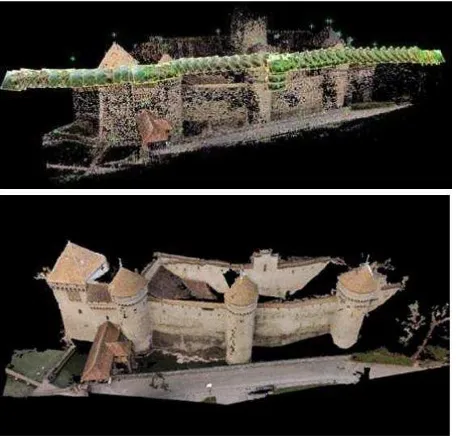
The Chillon Castle (Figure 1) is an island castle located on the shore of Lake Geneva, close to the city of Montreux. It consists of 100 independent, yet partly connected, buildings and is one of the most visited historic monuments in Switzerland.
Figure 1. The Chillon Castle
2.3 Surveying Equipment
2.3.1 GNSS Data: A Trimble R 10 GNSS receiver was used in
RTK‐mode using a virtual reference station for measuring 11 marked points two times in different satellite constellations. The mean difference between the two measurements was 10 mm in x and y and 20 mm in z. Some of the GCPs were visible in the images (as shown in Figure 3) and some of them were used to define the tachymetric network as described in following.
2.3.2 Tachymeter Data: A tachymetric network (Figure 2) was measured with a Trimble 5601 total station from the land side in order to survey control points which are measurable in both terrestrial and aerial images and detectable in the laser scan.
Figure 2. Tachymetric network for surveying the control and verification points
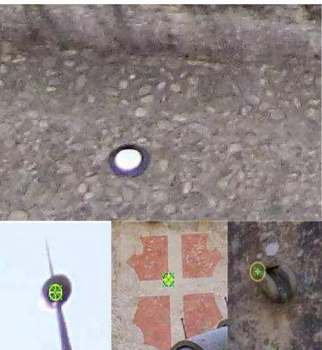
Figure 3. Marked control point and laser scan target from oblique aerial view (top). Natural control and verification points
from features (bottom)
Placing surveying marks on facades is strictly prohibited at the cultural heritage site. Instead, we used distinctive natural points of the buildings as control points (Figure 3). Most of the points were measured from different viewpoints with both instrument faces. For example, they could be surveyed with reflectorless distance or as spatial intersection without distance measurement (e.g. the spheroids on the top of the roofs). The least square adjustment leads to standard deviations of 8 mm, 7 mm and 6 mm, respectively, in x, y and z, taking the errors of the GNSS‐ points into account.
Figure 4. Results of tachymetric control and verification points
To acquire a comparable geodetic datum for the laser scan, 9 distinctive points from the tachymetric measurement were used, along with the laser scan targets, during registration of the scans. This resulted in the mean residuals of 2 mm for the laser targets and 10 mm for the tachymetric points after adjustment, which seems sufficient, considering the fact that the tachymetric points were not perfectly detectable in the gridded point cloud. Gross errors were removed manually from the registered scan result, and each point was in average 5 mm apart from the adjacent ones. The colored laser scan point cloud is shown in Figure 5 below.
Figure 5. Laser scan point cloud registered from three individual laser scans (blue points: laser scan targets, red points: tachymetric points). The registration was performed using the
bounded software provided with the laser scanner
2.4 Image acquisition and processing
For the cameras and lenses that possessed a manual setting option, the following settings were taken in order to keep a stable image-capturing condition:
No zooming for the lenses with variable focal length Manual focus setting once for all the images Physical image stabilization turned off Small ISO values to prevent ISO noise
Higher aperture values to get larger depth of field Tripod mount for all cameras except for the GoPro and
Phantom 2 vision datasets
The following processing was performed using Pix4Dmapper in default mode for processing and point cloud densification. Everything was calculated on a standard computer with 16 GB of RAM. rayCloud editor. The image view then automatically presents all the local image parts where this GCP can be seen side by side. This makes the GCP selection highly efficient and avoids opening and closing a lot of images.
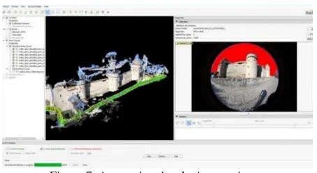
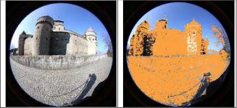
Multi-view stereo processing of terrestrial pictures tends to produce point clouds with errors in “densification of the sky.” Therefore, Pix4Dmapper implements an “Image Annotation” option. This is an automatic segmentation of the image, such that one can simply draw once around the outline of the measurable object to filter out the sky region seen in Figure 7. Since this cut affects rays to the infinity, there is no need to mark the annotation areas in all of the pictures.
Figure 6. Efficient marking of GCPs: the white light ray shows the measuring from the actual image
Figure 7. Annotating the sky in one picture
In the following, we will further describe the different datasets taken. For each camera, we give a short description and show the reconstruction. Table 1 shows the characteristics of the different datasets. The residuals of the GCPs are listed from south to north (left to right from the view of the land side facade) and grouped in GCPs on the facade to the land side.Above this facade, GCPs on top of the towers, on the backside of the facade (all natural distinctive points), and on the ground, are marked with plates, mainly for the aerial pictures, but partially also detectable in the terrestrial images.
2.4.1 Sony NEX 7: This image set surrounds the whole exterior of the castle. In front of the facade, different distances were used
Lens 16mm
Number of images 157 landside
152 seaside 376
1,690,661 2,781,688 3,675,673 1,186,377 207,311 1,540,623 864,360 309,390
Mean reprojection
error 0.16 pixels 0.28 pixels 0.24 pixels 0.18 pixels 0.13 pixels 0.12 pixels 0.43 pixels 0.46 pixels RMS error to all
in a quite limited space. In addition to the land-side pictures, images were taken from the lake-side using a boat. Because the lens was un-mounted from the body between lake-side and land-side images, variation in the interior parameters can be expected. Therefore, two different sets of camera parameters were calculated. To do this, two single Pix4Dmapper projects were generated and merged together after finishing the initial processing (bundle adjustment) for the two individual projects. The results of this and the dense point cloud are shown in Figure 8.
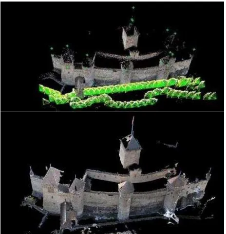
Figure 8. Results of the bundle adjustment. Automatic tie points, GCPs, and camera centres are shown in rayCloud Editor
(top) and the dense model at the bottom for the Sony Nex 7
2.4.2 Sony Alpha7R: The Sony Alpha7R has a 36MP full frame
CMOS sensor. Currently there are only a limited set of lenses available that support the full frame sensor. We used Sony 2.8/16mm fisheye lens with M-mount and the corresponding E-mount adapter to get the full 36MP image. All images have been taken with a tripod.
2.4.3 Canon 7D: Comparable to the NEX 7, this image set nearly surrounds the whole exterior, excluding a part in the north of the land-side, which has a bigger height difference and vegetation. In addition to the land-side pictures, which included images normal to the facade and oblique in horizontal and vertical orientation, there were also pictures taken from the facades on the lake-side using a boat, leading to a nearly closed circle around the facade.
2.4.4 Canon 6D: The Canon 6D has a 20.2MP full frame CMOS
sensor. An integrated GPS receiver tags geolocation into the EXIF data that was automatically used by Pix4Dmapper as an estimate of exterior positions.
Figure 9. Results of the bundle adjustment. Automatic tie points, GCPs, and camera centres shown in rayCloud Editor (top) and the resulting dense point cloud at the bottom for the
Canon 7D
Figure 10. Canon 6D with Sigma fisheye 8mm example. On the right one can see the automatically extracted and geometrically verified key-points after bundle adjustment. The distribution up
to the border of the image indicates the correctness of our fisheye camera model
very wide 3D range. This is the advantage we are searching for in indoor or city modelling.
Figure 11. Results of the bundle adjustment. Automatic tie points, GCPs, and camera centres shown in rayCloud Editor (top) and the dense point cloud (bottom) for the 8mm dataset
2.4.4.2 Fisheye Lens 10 mm: This set consists of normal looking pictures that were taken walking down the facade two times in slightly different distances. In addition, some images were taken from the north path out of the vegetation.
Figure 12. Results of the bundle adjustment. Automatic tie points, GCPs, and camera centres shown in rayCloud Editor
(top) and the resulting dense point cloud (bottom) for the 10mm lens dataset
2.4.4.3 Zoom Lens 28 mm: This image set consists of images directly in front of the wall, some pictures using the limited space behind the wall and also some images from the upper street. In addition to the normal images taken of the facade, oblique images of both sides in horizontal and vertical orientations were taken.
Figure 13. Results of the bundle adjustment. Automatic tie points, GCPs, and camera centres shown in rayCloud Editor
(top) and the dense point cloud (bottom) for the 28mm lens dataset
2.4.5 GoPro Hero3+: Using the GoPro Hero3+ (black edition)
Figure 14. Results of the bundle adjustment. Automatic tie points, GCPs, and camera centres shown in rayCloud Editor
(top) and the resulting dense point cloud (bottom)
2.4.6 Phantom 2 Vision: The Phantom2 Vision is a remotely controlled quadcopter. It ships with a 4000x3000 pixel camera that can be triggered from a mobile phone or at fixed intervals starting from 1 second. Similar to the GoPro, it has a wide angle fisheye lens. We captured the images by Phantom 2 Vision in remote-controlled flight mode with interval capturing of 1 second, while the Phantom Vision was used in time lapse mode taking an oblique picture every 3 seconds.
Figure 15. Results of the bundle adjustment. Automatic tie points, GCPs, and camera centres shown in rayCloud Editor
(top) and the resulting dense point cloud (bottom)
2.5 Comparison to terrestrial laser scanning
The final photogrammetric point cloud results were compared to the laser scan point clouds using the open-source software CloudCompare (CloudCompare). The visualizations show the distance to the reference data (laser scan) for each photogrammetric point cloud. Since different point clouds sample the underlying surfaces differently, simply calculating the distance to the closest point generally does not yield an accurate estimate of the distance between two surfaces. The distances were therefore obtained by first triangulating the
photogrammetric point clouds and then calculating the point‐ surface distance for every point of the laser scan cloud.
Table 2. Residuals of the used GCPs.
3. RESULTS AND DISCUSSION
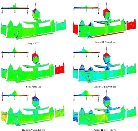
Figure 16 shows the color‐coded difference between the laser scan and the reconstructions of the different datasets as signed distances in the range [‐150 mm, 150 mm]. In the histograms, the distance for most points fall within this range. Some plots have large red areas. These do not represent reconstruction errors, but simply show that no data has been acquired in this area for the dataset in question.
The data sets from the NEX 7 (16 mm), Canon 7D (20 mm) and Canon 6D (28 mm) show an obvious systematic error in the areas where single laser scan stations are registered. The point cloud registration of the scan station in the north, which is quite near to the end of the wall, doesn’t seem to be sufficient, and the area in the very north shows identical errors up to 4 cm. Besides the imperfect scan registration in these areas, the scanner rays were reflected in an acute angle from the surface, which possibly also had an effect on the results.
The parts of the building with a normal surface pointing more to the scan station, like the building projection at the bottom in the
north area or the parts of the last small tower facing to the scan station, have small differences of up to 10 mm.
For all datasets, we fitted a Gaussian to the deviation histograms and estimated the mean and standard deviation.
Table 3 summarizes these results. For all datasets, the mean is significantly lower than the standard deviation, indicating that the results are identical within their error. The datasets taken with a
tripod have the lowest deviations, followed by the Phantom2 Vision. The fisheye lenses mostly reach good accuracies; when the field of view was not too large, no significant degradation in accuracy could be detected compared to a perspective lens. The 8 mm fisheye has the highest deviation, indicating that the 180-degree field of view introduces a larger error. For the GoPro Hero3+, the rolling shutter also contributes to the overall error, making it less accurate.
Table 2 shows the results of the bundle adjustment. The standard deviation of the GCPs is in the range of a few millimeters and comparable for all cameras. The projection and xyz-errors show a clear increase for the two rolling shutter cameras (GoPro and Phantom2 Vision). While the projection error of the global shutter cameras is around 0.5, the rolling shutter cameras have an error of 2 or 3 pixels. Taking the rolling shutter into account in the mathematical model would most likely decrease this error.
Sony NEX 7 Canon7D 20mm lens
Sony Alpha-7R Canon 6D fisheye 8mm
Phantom Vision fisheye GoPro Hero3+ fisheye
Figure 16. Color coded difference between the laser scan points and the photogrammetric triangulated meshes (red and blue values indicate missing data for the photogrammetric point cloud)
Table 3. Comparison of the different datasets to the laser scan data, which in its highest point sampling mode required
an acquisition time of ~4 hours. The deviation to laser corresponds to a Gaussian fit of the deviation histograms in
4. CONCLUSION
We compared photogrammetric 3D models from images of different cameras and lenses with the results of a laser scanner. The accuracy of image-derived 3D models is generally comparable to that of a laser scanner, but with a large advantage of ease of use, highly reduced acquisition time (4 hours for the laser scan, 10 minutes for the GoPro), and cost. A comparison of different perspective and fisheye lenses was done to investigate the influence of their smaller and non‐uniform GSD to see if it outweighs the clear advantage for image based 3D modelling (i.e. better performance in poorly-textured indoor scenarios as well as flexibility in capturing a complex scene with a very limited distance to the scene).
From the experiments one can conclude that even fisheye lenses can reach accuracies that are substantially below 10cm for an approximate object distance of 15m. The worst result is obtained from a full 180-degree lens, while the less extreme fisheye lenses on the Phantom2 Vision and for the GoPro have results that are additionally disturbed by their rolling shutters and the fact that they have been triggered in a handheld situation. This was done on purpose to show their accuracy when the acquisition time is as fast as possible. Our experience shows that the quality of both the Phantom and GoPro increases when the cameras are mounted on a tripod or when the rolling shutter is accounted for in the camera model.
The presented scenario shows that while the accuracy of a full 180-degree fisheye is not as good as that of a perspective lens, smaller angle fisheye lenses on good cameras give comparable results to perspective lenses. The rolling shutter of consumer cameras has an additional effect, which makes the comparison more difficult.
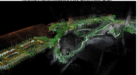
For indoor scenarios as shown in Figure 17, perspective cameras would be impractical. Fisheye cameras yield very good results in this indoor situation.
REFERENCES
C. Strecha, W. von Hansen, L. Van Gool, P. Fua and U. Thoennessen, 2008. On Benchmarking Camera Calibration and Multi-View Stereo for High Resolution Imagery [Journal]. - [s.l.] : Proceedings of the IEEE Conference on Computer Vision and Pattern Recognition
C. Strecha, T. Pylvanainen, and P. Fua, 2010. Dynamic and Scalable Large Scale Image Reconstruction [Conference] // CVPR.
C. Strecha, T. Tuytelaars, and L. Van Gool, 2003. Dense Matching of Multiple Wide-baseline Views [Conference]. - [s.l.] : Proceedings of the International Conference on Computer Vision (ICCV)
C. Strecha, L. Van Gool and P. Fua, 2008. A generative model for true orthorectification [Conference] // Proceedings of theInternational Society for Photogrammetry and Remote Sensing (ISPRS). - Bejing : [s.n.]
CloudCompare [Online]. - http://www.danielgm.net/cc/. Hughes, C. [et al.], 2010. Accuracy of fish-eye lens models [Journal] // Applied Optics. - 17 : Bd. 49. - S. 3338-3347. J. Kannala and S.S. Brandt, 2006. A generic camera model and calibration method for conventional, wide-angle, and fish-eye lenses [Journal] // IEEE Transactions on Pattern Analysis and Machine Intelligence. - 8 : Bd. 28. - S. 1335-1340.
Pix4D [Online], 2014. - September 2014. - www.pix4d.com. S. Agarwal, Y. Furukawa, N. Snavely, B. Curless, S.M. Seitz, and R. Szeliski, 2012. Reconstructing Rome [Journal] // Computer vol 43, no 6. - 2012. - S. 40.47.