Monitoring High-frequency Ocean signals using low-cost GNSS/IMU buoys
Yu-Lun Huang a, Chung-Yen Kuo a, Chiao-Hui Shih a, Li-Ching Linb, Kai-wei Chiang a, Kai-Chien Cheng c
a Department of Geomatics, National Cheng Kung University, Tainan City 701, Taiwan - (P66034133, kuo70, P66024015, kwchiang)@mail.ncku.edu.tw
b International Wave Dynamic Research Center National Cheng Kung University, Tainan City 701, Taiwan - [email protected] c Dept. of Earth and Environmental Sciences, National Chung Cheng University, Chiayi, Taiwan - [email protected]
Commission VIII, WG VIII/9
KEY WORDS: Global Navigation Satellite System (GNSS) buoys, Inertial Measurement Unit (IMU), tide gauge
ABSTRACT:
In oceans there are different ocean signals covering the multi-frequencies including tsunami, meteotsunami, storm surge, as sea level change, and currents. These signals have the direct and significant impact on the economy and life of human-beings. Therefore, measuring ocean signals accurately becomes more and more important and necessary. Nowadays, there are many techniques and methods commonly used for monitoring oceans, but each has its limitation. For example, tide gauges only measure sea level relative to benchmarks and are disturbed unevenly, and satellite altimeter measurements are not continuous and inaccurate near coastal oceans. In addition, high-frequency ocean signals such as tsunami and meteotsunami cannot be sufficiently detected by 6-minutes tide gauge measurements or 10-day sampled altimetry data. Moreover, traditional accelerometer buoy is heavy, expensive and the low-frequency noise caused by the instrument is unavoidable. In this study, a small, low-cost and self-assembly autonomous Inertial Measurement Unit (IMU) that independently collects continuous acceleration and angular velocity data is mounted on a GNSS buoy to provide the positions and tilts of the moving buoy. The main idea is to integrate the Differential GNSS (DGNSS) or Precise Point Positioning (PPP) solutions with IMU data, and then evaluate the performance by comparing with in situ tide gauges. The validation experiments conducted in the NCKU Tainan Hydraulics Laboratory showed that GNSS and IMU both can detect the simulated regular wave frequency and height, and the field experiments in the Anping Harbor, Tainan, Taiwan showed that the low-cost GNSS buoy has an excellent ability to observe significant wave heights in amplitude and frequency.
1. INTRODUCTION
Ocean signals, including tsunami, meteotsunami, storm surge, as sea level change, and currents, are covering the multi-frequencies in oceans. These signals have the direct impact on the life and societal benefit of human-beings. To measure ocean signals accurately becomes more and more important and necessary. Nowadays there are many techniques commonly used for monitoring oceans such as tide gauges and satellite measurements are not continuous and inaccurate in coastal regions because of noisy radar waveforms and unreliable geophysical corrections (Lee et al. 2010). In addition, due to lack of high sampling rate, high-frequency ocean signals such as tsunami and meteotsunami cannot be detected by 6-minutes tide gauge measurements or 10-day sampled altimetry data. Moreover, traditional accelerometer buoy is generally heavy, large, and expensive and the low-frequency error caused by the instrument is unavoidable. Because of these reasons, the GNSS buoy has been introduced.
GNSS buoy equipped with a dual- or triple-frequency GNSS receiver is appropriate to collect high-frequency sea surface information and the accuracy of it can reach several cm(s) level. Other advantages are less expensive, lightweight and small volume that can be easily hand-deployed for conducting the experiments. However, there are still some drawbacks of GNSS buoy. Because of the GNSS signals shielded by field environments, the unavoidable cycle slips and signal loss lead
to GNSS outages. In addition, the randomly tilt motion caused by waves or winds decreases the positioning accuracy. In order to solve these problems, we develop a low-cost GNSS buoy equipped with a self-assembled IMU to promote the accuracy of positioning when the GNSS signal is poor or interrupted and also to correct the buoy tilt to acquire vertical heights.
In this study, we used a small, low-cost and self-assembly autonomous IMU that independently collects continuous acceleration and angular velocity data to provide the kinematic position information during the GNSS outages and correct the tilt motions by the orientation information. The main idea is integrate the Differential GNSS (DGNSS) or Precise Point Positioning (PPP) solutions with IMU data. Likewise, we evaluate the accuracy of GNSS buoy vertical positioning from different GNSS software such as GAMIT/TRACK, GIPSY and GRAFNAV processed by DGNSS and PPP techniques. Furthermore, we also analysed the ability of calculating the wave heights from IMU measurements and compared with the wave gauge data.
In our experiments, the validation experiments and field experiments were conducted in the NCKU Tainan Hydraulics Laboratory and Anping Harbor, Tainan, respectively.
are two types of GNSS observations. Equations (1) and (2) are
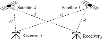
where P is the pseudo-range observation; is the carrier phase observation; is double difference; is the true geometric distance between the receiver and the satellite; dtropis the tropospheric delay; dionis the ionospheric delay; is the wave length of carrier phase; N is the ambiguity of the carrier phase; and is other sources of noise and bias. Figure 1 shows the illustration of the DGNSS technique.
Figure 1. DGNSS technique (Tseng et al. 1999)
2.2 PPP technique
Because the positioning accuracy of DGNSS technique is restricted to baseline length, PPP technique is used to overcome these limitations of DGNSS. The observation functions of PPP are composed of un-difference measurements and the amounts of them are much more than the difference ones. But unlike DGNSS, the model of PPP is more complicated and the number of parameters to be estimated are much more. Equations (3) and (4) are the pseudo-range and carrier phase observations (Abdel-Salam et al. 2002).
carrier phase observation; Li is the carrier with frequency fi; dt
is the satellite clock error; dT is the receiver clock error; do rb is
the satellite orbit error; dmuly/P(Li) and dmult/(Li) are the multipath effects. Figure 2 shows the illustration of the PPP technique.
Figure 2. PPP technique (Tseng et al. 1999)
acceleration data
As we know, the displacement, velocity and acceleration data could be changed between time domain and frequency domain. At first, performing the Fast Fourier transform (FFT) to change the acceleration data from time domain to frequency domain.
Then, multiplying the acceleration data by 1/2 to shift the acceleration data to displacement and performing Inverse Fourier Transform (IFFT) to get the displacement in time domain. Equations (5) shows the details of this method.
) displacement in frequency domain; is the circular frequency and f is the frequency.
However, the acceleration observations are influenced by the position and tilt angle of buoys, electronic interference, signal error and other factors, and the observations contain the noises in low-frequency band (Huang, 1998). In addition, multiplying
the acceleration data in frequency domain by 1/2 would cause the power of displacement to become much bigger than the acceleration one. Especially when the value of is small,
3. INTRODUCTION OF INSTRUCMENTS AND EXPERIMENTS
3.1 GNSS buoy
GNSS buoy is an instrument that collect high samples data of sea level height regularly. Kelecy et al. (1994) improved that using the lightweight GNSS buoy to collect the mean sea surface data had the similar effects as the big one did, but it needed extra sources of power supply. In this study, we used the Waverider GNSS Buoy shown in Figure 3. It was simple-structure, less-expensive and using a lifebuoy as the vehicle which can be reused. Moreover, it was assembled with a dual-frequency geodetic-grade Trimble R4 GNSS receiver to get the results of vertical positioning, and a self-assembly autonomous IMU was applied to enhance the accuracy of positioning during the outages of GNSS instrument and calculate the wave heights.
Figure 3. Waverider GNSS/IMU buoy
3.2 Validation experiment
Before conducting the field experiment in the coastal area, the validation experiment was conducted in the NCKU Tainan Hydraulics Laboratory. In this experiment, the wave gauge and the GNSS Buoy were set on the tank to measure the wave synchronously. And the wave generator made five quantitative regular waves with the wave period of 3 seconds and the wave heights were from 20cm to 50cm. The main idea of the experiments was to analyse whether GNSS or IMU can detect the simulated regular wave frequency and height. Figure 4 show the scenes of the experiment.
Figure 4(a). Numerical wave tank and wave gauge.
Figure 4(b) Waverider Buoy in the wave tank
3.3 Field experiment
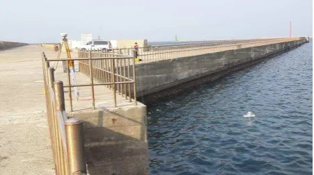
In this study, the field experiment was conducted in the south bank of Anping Harbor, Tainan, Taiwan, in the daytime on 27 November of 2014. One GNSS receiver was established on the shore as a reference station and another GNSS receiver was installed on the GNSS buoy to continuously collect the sea surface information. Figure 5 shows the in-situ arrangement of the field experiment.
Figure 5. In-situ arrangement of experiments in Anping Harbor.
4. RESULTS OF EXPERIMENTS
4.1 Results of validation experiments
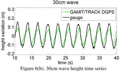
The GNSS results of the experiment in the wave tank as shown in Figure 6 indicate that the height variations measured by GNSS can almost fit the wave gauge properly only when the wave height reach 40 or 50cm, as some differences appear between two of them.
Figure 6(a). 20cm wave height time series
GNSS
Figure 6(b). 30cm wave height time series
Figure 6(c). 40cm wave height time series
Figure 6(d). 50cm wave height time series
In the FFT power spectrum part of results, no matter what the wave height is, the peak value of the GNSS and the wave gauge are both one-third Hz which are corresponding to the regular wave with the period of 3 seconds. Therefore, it means that the GNSS has the capability to detect the regular wave frequency. Figure 7 show the results of FFT power spectrum in different wave height, respectively.
Figure 7(a). 20cm wave height FFT power spectrum
Figure 7(b). 30cm wave height FFT power spectrum
Figure 7(c). 40cm wave height FFT power spectrum
Figure 7(d). 50cm wave height FFT power spectrum
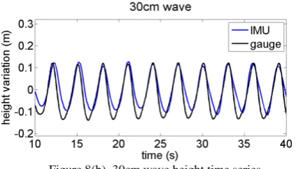
Like the results of GNSS, the IMU results in Figure 8 show the similar results as GNSS only when the wave height reach 40 or 50cm, as some differences appear between two of them.
Figure 8(b). 30cm wave height time series
Figure 8(c). 40cm wave height time series
Figure 8(d). 50cm wave height time series
Similar to the results of GNSS, no matter what the wave height is, the peak value of the IMU and the wave gauge are one-third Hz which are corresponding to the regular wave with the period of 3 seconds. It means that the IMU has the capability to detect the regular wave frequency. Figure 9 show the results of FFT power spectrum in different wave height, respectively.
Figure 9(a). 20cm wave height FFT power spectrum
Figure 9(b). 30cm wave height FFT power spectrum
Figure 9(c). 40cm wave height FFT power spectrum
Figure 9(d). 50cm wave height FFT power spectrum
4.2 Results of field Experiments
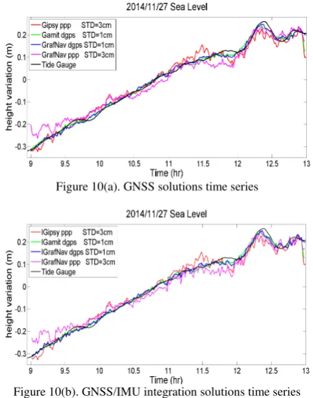
Figure 10(a). GNSS solutions time series
Figure 10(b). GNSS/IMU integration solutions time series
In contrast to the open sea wave gauge data as shown in Table 1, the GNSS, IMU and GNSS/IMU integration solutions had the obvious peak value near the 0.1 Hz in the FFT power spectrum, which were corresponding to the average wave frequency recorded by wave gauge. It meant that the GNSS/IMU buoy has the ability of observing the wave in frequency. Figure 11 show the FFT power spectrum of GNSS, IMU and GNSS/IMU integration solutions.
Table 1. Wave frequency of Anping wave gauge observations on November 27, 2014.
2014/11/27 Wave frequency (Hz) of wave gauge observations
Time(Hr) Frequency (Hz)
9 0.200
10 0.200
11 0.179
12 0.175
13 0.175
Average 0.187
Figure 11(a). FFT power spectrum of GNSS solutions
Figure 11(b). FFT power spectrum of IMU solutions by High-pass filter and Gaussian filter.
Figure 11(c). FFT power spectrum of integration solutions
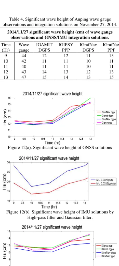
Tables 2, 3, 4 and Figure 12 show the significant wave heights derived from GNSS, IMU and GNSS/IMU integration solutions that compare with the open sea wave gauge data, respectively. The results of wave gauge showed that the wave height increased from 9 am to 11 am and decreased from 11 am to 1 pm. However, the location of GNSS buoy was far from the open sea that couldn’t clearly observe the real trend of wave height changing like the wave gauge did. Therefore, it meant that the GNSS/IMU cannot obviously observe the significant wave height in trends in this study.
Table 2. Significant wave height of Anping wave gauge observations and GNSS solutions on November 27, 2014.
2014/11/27 significant wave height (cm) of wave gauge observations and GNSS solutions.
Time (Hr)
Wave gauge
GAMIT DGPS
GIPSY PPP
GrafNav DGPS
GrafNav PPP
9 44 12 12 12 12
10 42 12 12 12 12
11 40 12 13 12 12
12 43 14 15 14 14
13 47 16 15 15 15
Table 3. Significant wave height of Anping wave gauge observations and IMU solutions on November 27, 2014.
2014/11/27 significant wave height (cm) of wave gauge observations and IMU solutions.
Time (Hr)
Wave gauge
0.0325 Hz High-pass filter
0.0325 Hz Gaussian filter
9 44 28 19
10 42 17 13
11 40 19 14
12 43 25 19
Table 4. Significant wave height of Anping wave gauge observations and integration solutions on November 27, 2014.
2014/11/27 significant wave height (cm) of wave gauge observations and GNSS/IMU integration solutions.
Figure 12(a). Significant wave height of GNSS solutions
Figure 12(b). Significant wave height of IMU solutions by High-pass filter and Gaussian filter.
Figure 12(c). Significant wave height of integration solutions
5. CONCLUSIONS AND SUGGESTIONS
In this study, a low-cost self-assembled GNSS/IMU buoy was used to monitor the high-frequency ocean signals. The main idea is integrating the DGNSS or PPP solutions with IMU data to improve the poor accuracy of positioning when GNSS signals are loss or randomly tilt motion of buoy caused by winds and waves. In the beginning, we conducted the validation experiment to analysis the quality of our GNSS and IMU instruments. It showed that the GNSS and IMU were capable to detect the regular wave height and frequency only when the wave height increased, there would exist a little differences to the referenced tide gauge data. After conducting the validation experiment, we performed the field experiment in Anping
Harbor, Tainan, and compared with the in-situ tide gauge and wave gauge measurements. In the GNSS solutions, both the accuracy of DGNSS and PPP solutions could reach cm level, and the DGNSS one was better than the PPP one. Comparing to the wave height and frequency data of the wave gauge, the GNSS/IMU buoy could not obviously observe the significant wave height in trends because the location of the buoy was far from the open sea. However, the GNSS/IMU buoy had the excellent ability on observing the wave in frequency.
On the other hand, the results of GNSS/IMU integration solutions were limited by the high accuracy of original GNSS solutions and the eased ocean environment of inner harbour. Therefore, the improvement by integrating GNSS and IMU techniques was restricted. Maybe in the future, we could perform the buoy field experiments in the open sea to get more accurate results compared to the wave gauge measurements.
ACKNOWLEDGEMENTS
This work is supported by the Ministry of Science and Technology of Taiwan (No. MOST 103-2221-E-006-115 and No. MOST 105-2911-I-006-301) and the International Wave Dynamics Research Center of National Cheng Kung University for providing financial support. We acknowledge the Inter-disciplinary Research Division, Harbor and Marine Technology Center for the assistance to collect GPS buoy data in the Anping Harbor.
REFERENCES
Abdel-Salam, M., Y. Gao, and X. Shen, 2002. Analyzing the performance characteristics of a precise point positioning system. Proceedings of the ION GPS-2002, Oregon Convention Centre, Portland, Oregon, USA, September 24-27.
Cheng, K. C., 2004. GPS Buoy Campaigns for Vertical Datum Improvement and Radar Altimeter Calibration. OSU Report No.470, Geodetic Science and Surveying in the Department of Civil and Environmental Engineering and Geodetic Science, The Ohio State University, Columbus, Ohio, USA.
Cheng, K. C., 2005. Analysis of Water Level Measurements carrier-phase point positioning with precise orbit products. Proceedings of the KIS 2001, Banff, Alberta, Canada, June 5-8.
duction to GAMIT/GLOBK. Department of Earth, Atmospheric, and Planetary Sciences, Massachusetts Institute of Technology, Cambridge, Massachusetts, USA.
Huang, M. C., 1998. Time domain simulation of data buoy motion. Proceedings National Science Council ROC(A) Vol. 22, 6, pp. 820-830.
Jet Propulsion Laboratory Group, 2015. GIPSY-OASIS User Guide, California, USA.
Johnson, D., R. Stocker, R. Head, J. Imberger, and C. Pattiaratchi, 2003. A compact, low-cost GPS drifter for use in the oceanic nearshore zone, lakes, and estuaries. J. Atmos.
Oceanic Technol., 20, 1880–1884.
Kuo, C. Y, K. W. Chiu, K. W. Chiang, K. C. Cheng, L. C. Lin, H. Z. Tseng, F. Y. Chu, W. H. Lan, and H. T. Lin, 2012. High-Frequency Sea Level Variations Observed by GPS Buoys Using Precise Point Positioning Technique, Terr. Atmos. Ocean. Sci., 23(2), pp. 209-218.
Lee, H., C. K. Shum, W. Emery, S. Calmant, X. Deng, C. Y. Kuo, C. Roesler, and Y. Yi, 2010. Validation of Jason-2 altimeter data by waveform retracking over California coastal ocean. Mar. Geodesy, 33, pp. 304-316.
Lin, L.C., Liang, M.C. and Chang, H.K., 2010. Periods of 10-30 Minutes of Sea Level Variation Observed in the Coastal Regions of Taiwan. In: European Geosciences Union General
Assembly 2010. Geophysical Research Abstracts Vol. 12,
EGU2010-3138-1.
National Data Buoy Center (NDBC), 2015. How are significant wave height, dominant period, average period, and wave steepness calculated. Mississippi, USA. http://www.ndbc.no-aa.gov/wavecalc.shtml (3 Nov. 2015)
Tseng, C. L., C. M. Chu, 1999. GPS Satellite Surveying Principles and Applications. Second Edition, Satellite Geo-information Research Center, National Cheng Kung University, Tainan, Taiwan (R.O.C.)
Way Point Product Group, 2015. GrafNav/GrafNet User Guide. Canada.
Willis, J. K., D. P. Chambers, C. Y. Kuo, and C. K. Shum, 2010. Global sea level rise: Recent progress and challenges for the decade to come. Oceanography, 23, pp. 26-35.
Yeh, T. K., C. Hwang, J. F. Huang, B. F. Chao, and M. H. Chang, 2011. Vertical displacement due to ocean tidal loading around Taiwan based on GPS observations. Terr. Atmos. Ocean. Sci., 22, pp. 373-382.
Zumberge, J. F., M. B. Heflin, D. C. Jefferson, M. M. Watkins, and F. H. Webb, 1997. Precise point positioning for the efficient and robust analysis of GPS data from large networks. J.