How do Broader Monetary Aggregates and
Divisia Measures of Money Perform in
McCallum’s Adaptive Monetary Rule?
Saranna Robinson Thornton
This paper addresses two questions. First, can a monetary policy rule be identified that; (1) promotes greater levels of price stability than actual discretionary policy has, (2) performs well (i.e., promotes long-run price stability) in different, plausible macroeconomic mod-els, (3) performs well when financial innovations, regulatory changes or other factors alter the relationship (e.g., velocity) between the policy instrument and the target variable, (4) when relevant, performs well when financial innovations, regulatory changes, or other factors alter the relationship between the control variable and the policy instrument, (5) allows the public to monitor central bank compliance with the rule, and (6) is operational?
Second, can adaptive rules using broader Divisia measures of money as policy instruments (e.g., M2 and above) achieve greater levels of price stability than rules using the traditional monetary aggregates? Divisia measures of money are examined because research suggests they may exhibit a stronger and more stable relationship with nominal GDP than broad monetary aggregates computed as the unweighted sum of their compo-nent assets.
Rules that indirectly target a stable price level are examined using the traditional aggregates and Divisia measures of M2, M3, and Liquidity (L), respectively, as policy instruments. Counterfactual GDP simulations are conducted in three different macroeco-nomic models over the time period 1964:Q2–1997:Q4. The performance of rules using the different policy instruments is assessed by comparing the simulated GDP time path to a target time path consistent with long-run price stability. All simulations explicitly assume that the Fed cannot precisely control the policy instruments over time periods as short as one quarter.
Department of Economics Hampden-Sydney College Hampden-Sydney, Virginia.
Address correspondence to Dr. S. R. Thornton, Department of Economics, Hampden-Sydney College, Hampden-Sydney, VA 23943.
Results suggest that all the policy instruments examined satisfy the six criteria for rule success. The best performance is produced by the rule using Divisia L as its policy instrument. Rules using Divisia measures of money usually outperform their (traditional) monetary aggregate counterparts—although the difference is often inconsequential. © 2000 Elsevier Science Inc.
Keywords: Monetary policy rule JEL classification: E42; E52
I. Introduction
Over the last twenty years an increasing number of economists and policy makers have come to agree that the primary goal of monetary policy should be price stability. Yet, in a world characterized by changing structural relations between policy instruments and ultimate goals, as well as other uncertainties, a question remains. What is the most appropriate means to achieve price stability? Should central bankers use discretionary monetary policy— or policy rules?
Proponents of discretionary policy argue that central bankers need a high degree of flexibility in order to respond to random shocks or changes in structural relationships— both of which may cause macroeconomic variables to deviate from policy goals. Sup-porters of rules argue that: (1) discretionary policy is likely to succumb to an inflationary bias when the central bank’s objective function negatively weights inflation and positively weights levels of output above the full-employment level,1(2) central bank commitment to a policy rule capable of ensuring long-run price stability will eliminate that inflationary bias, and (3) adaptive rules incorporating feedback terms can provide a sufficiently flexible response to accommodate random shocks as well as changes in structural relationships between a policy instrument and goal variable.
A successful monetary policy rule meets the following criteria. The rule should; (1) promote greater levels of price stability than actual discretionary policy has, (2) perform well (i.e., promote long-run price stability) in different, plausible macroeconomic models, (3) perform well when financial innovations, regulatory changes or other factors alter the relationship (e.g., velocity) between the policy instrument and the target variable, (4) when relevant,2 perform well when financial innovations, regulatory changes, or other factors alter the relationship between the control variable and the policy instrument, (5) allow the public to monitor central bank compliance with the rule, and (6) be operational. This paper addresses two questions. First, can one or more monetary policy rules be identified that meets the six criteria above? Thornton (1998, 1999) suggests that an M2 version of McCallum’s Rule meets all six criteria, but it would be useful for policymakers to know if other policy instruments would perform equally as well in a McCallum-type
1Monetary policy under the Volcker- and Greenspan-led Fed doesn’t contradict theory. During this time the Fed has succeeded in achieving inflation stability—not price stability. Also, recent success in achieving inflation stability is not invariant to the membership of the FOMC.
rule. In an attempt to answer this question, the performance of six versions of McCallum’s adaptive rule are evaluated from 1964:Q2–1997:Q4. Each rule indirectly targets a stable price level through an explicit nominal GDP target and uses a different monetary variable as its policy instrument.
Rules utilizing some other commonly proposed, non-monetary, instruments are not evaluated because research indicates that they may not be suitable policy instruments based on the six criteria listed above. For example, Friedman (1988) finds that rules utilizing measures of reserves typically don’t ensure long-run price stability. McCallum (1998) and Judd and Motley (1992) both find instances where interest rates don’t perform well as a policy instrument in a rule targeting a stable price level. Clark (1994) finds that neither the variability of real GDP growth or inflation are reduced by an interest rate rule targeting a stable inflation rate.3
Some monetary variables are also not considered here as potential policy instruments because prior research shows they do not meet the six criteria above. Thornton (1998, 1999) found that the monetary base is sub-optimal because its performance (in rules targeting levels of nominal GDP) is not robust across different economic models.
Economists compute the traditional monetary aggregates as the unweighted sum of the dollar amounts of the different assets included in the aggregate (e.g., M1, M2, M3, etc.).4 However, the equal weighting of different assets is only appropriate if the assets included in a given monetary variable are perfect substitutes for each other. Clearly this is not the case for broader measures of money such as M2 and M3. It has been suggested that a superior theoretical and empirical definition of money is obtained by using a Divisia monetary index.5
Financial innovations and regulatory changes during the last three decades sometimes caused structural changes in the relationship between growth rates in some monetary aggregates (e.g., M2) and growth rates in GDP. Thornton and Yue (1992) suggest that because Divisia money represents the flow of monetary services provided by the assets included in a given monetary aggregate, the structural relationship between a Divisia measure of money and GDP may be less affected by financial innovations. If so, Divisia measure of money might be better policy instruments than the monetary aggregates. Thus, the second question this study asks is; can adaptive rules using broad Divisia measures of money (e.g., Divisia M2) as policy instruments perform better than rules using the corresponding monetary aggregates (e.g. M2)?
Narrower measures of money (e.g., Divisia M1, Divisia M1A, M1 and M1A) are not considered as policy instruments here. Thornton (1999) finds that versions of McCallum’s rule using these narrower measures of money as policy instruments do not meet the six criteria for rule success. Specifically, as noted by Feldstein and Stock (1993) the narrower
3The performance of interest rate rules in Clark (1994) seems inconsistent with the Fed’s recent experience using the federal funds rate to target a constant inflation rate. This may be due to the specification of interest rate rules. They typically include one feedback term that alters the policy instrument in response to a deviation from the rule’s nominal income target—but no explicit feedback term to directly adjust the policy instrument in response to structural changes in the relationship between interest rates and GDP. McCallum (1998) examines reasons behind central bankers’ attention to interest rate rules such as the one proposed by Taylor (1993).
monetary aggregates do not exhibit a strong and stable enough relationship with nominal GDP and thus the performance of rules using these variables as policy instruments is not robust for different macroeconomic models. Moreover, at the narrower levels of aggre-gation (e.g., M1 or M1A) the monetary assets included in the monetary variable are close enough substitutes for each other that graphically there is not much difference between the monetary aggregate and the respective Divisia measure of money. Thus, given the weaker relationship between narrower monetary aggregates and nominal GDP, it is not surprising that Divisia M1 and Divisia M1A are also unsuitable policy instruments.
Rules examined here use unweighted aggregates and Divisia measures of M2, M3 and Liquidity (i.e., L), respectively, as policy instruments.6A rule utilizing M2 is examined because research by Feldstein and Stock (1993) and Thornton (1993, 1998, 1999), etc., suggests it meets the six key criteria listed above. The performance of rules using the monetary aggregates and Divisia measures of M2, M3, and L, respectively, are compared in order to assess the hypothesis that the method of measuring the monetary services provided by a given policy instrument has a consequential impact on the outcomes of policy rules. If Divisia measures of money exhibit a more stable relationship with nominal GDP, rules using these variables as instruments may outperform rules using the corre-sponding monetary aggregates.
Section 2 reviews some issues in the choice of policy instruments. Section 3 explains the GDP simulation procedures utilized to evaluate rule performance.7Simulation results are derived assuming that the Fed cannot precisely control the policy instrument over periods of time as short as one quarter. Section 3 compares the performance of the policy rules to assess; (1) whether or not a given rule meets the six criteria for success, and (2) the robustness of rule performance to the method of measuring monetary services provided by a respective policy instrument. Section 4 evaluates the policy implications of GDP simulations and considers caveats bearing on any final assessment regarding the success of a particular rule. A conclusion follows.
Results suggest that during the sample period, 1964:Q2–1997:Q4, M2, M3, and L rules, using the monetary aggregates or Divisia measures of money, consistently meet the six criteria for success. Rules using Divisia measures of money almost always outperform their non-Divisia counterparts—although the difference is often inconsequential.
II. Some Issues in the Choice of a Policy Instrument
8Concerns regarding the public’s ability to monitor central bank compliance with a rule (i.e., transparency issues) emerge if the Fed doesn’t accurately control the policy instru-ment in the short-run. Although short-run control of the monetary aggregates and Divisia monetary variables would be imprecise, as Thornton (1998, 1999) notes, compliance with a rule using these variables as policy instruments might be gauged by establishing a narrow error band for the specified, quarterly policy instrument target level, as is commonly done with bilateral exchange rates under fixed exchange rate regimes. Levels
6Neither monetary aggregates or Divisia measures of M2, M3 or L are variables under the direct and precise control of the Fed. These six monetary variables are treated as instruments for achieving a nominal income target—assuming there is some other control variable (e.g., the federal funds rate or the monetary base) that the Fed can use to target each of them.
7All simulations utilize rules that target nominal GDP. Hereafter, the term ‘M2 rule’ or ‘Divisia M2 rule’ refers not to the rule’s target, but to its policy instrument.
of the policy instrument could be allowed to deviate from any given quarter’s target by the absolute value of a pre-specified, small percentage. Or, compliance could be measured by requiring the Fed to limit deviations from rule-specified policy instrument growth rates (measured in quarterly logarithmic units) to be zero on average with a mandated, relatively narrow, variance. This method of assessing compliance compares to the way the Fed measures bank compliance with reserve requirements. The specified compliance period could be a longer period of time (e.g., 1 year). The size of the error band in the first measure of compliance or the variance and compliance period in the second measure must be large enough to accommodate the normal range of money control error, but small enough to prevent discretionary policymaking.
An operational issue that arises from using policy instruments that the Fed can’t control precisely is that deviations of money growth from the quarterly, rule-prescribed targets may generate substantially greater deviations of nominal GDP from its target path. As Thornton (1998, 1999) demonstrates for McCallum’s Rule this problem is mitigated if (1) money control errors exhibit a systematic, negative, contemporaneous correlation with GDP shocks; and/or (2) the impacts of the money control errors are significantly offset by the rule’s feedback properties.
Feldstein and Stock (1993) note that the existence of a sufficiently strong and stable relationship to nominal income is another important factor affecting the performance of a policy instrument. Absolute stability in velocity growth is not necessary for McCallum’s rule to succeed. However, a more stable relationship between a policy instrument and GDP enhances rule performance.9
Although Feldstein and Stock (1993) conclude M2 is the preferred policy instrument in an adaptive rule, they don’t incorporate the impacts of imprecise control over M2 in their GDP simulations—arguing instead that the Fed could take steps to substantially increase its control over M2. Yet, to thoroughly appraise the likely success of a monetary variable in the role of policy instrument, one must consider more than the impacts of GDP shocks and changing structural relationships between the policy instrument and the GDP target. One must also simultaneously evaluate the impacts of random shocks that affect the linkage between the control variable (e.g., the federal funds rate or the monetary base) and the policy instrument.
A combination of several factors determines the success of a policy instrument. Some potential instruments (e.g., the monetary base, the federal funds rate) are controllable by the Fed in the short-run, but other policy instruments (e.g., M2) exhibit a stronger and more stable linkage to nominal income. Thornton (1998, 1999) finds it is the latter characteristic that is more important in determining the success of McCallum’s rule. The rule quickly corrects the effects of missed money targets on GDP targets—if there is a relatively strong and stable relationship between the policy instrument and GDP. On the other hand, missed GDP targets caused by shocks to GDP or other sources cannot be
easily offset if the policy instrument exhibits a weak and erratic relationship with nominal income.
Orphanides (1998) examines another operational issue affecting rules that target nominal GDP. Because of various data collection problems, nominal GDP figures are subject to frequent revisions and reasonably correct values of last quarter’s GDP aren’t available to Fed staff until the last few weeks of the current quarter. For at least 3 more years that “final estimate” will be subject to further revisions— often made in July of each year. And still more revisions may follow over longer time intervals.
Differences between the preliminary GDP estimate (which might be used by a policy maker to implement the rule) and the final estimate or the ultimate revision can be substantial. This informational problem introduces another source of error into rule implementation and the GDP simulations of rule performance. A policymaker, basing monetary policy on the Bureau of Economic Analysis’s preliminary estimate of last quarter’s GDP, will probably alter the policy instrument by a sub-optimal amount—if the preliminary estimate of last quarter’s GDP is not equal to the most accurate, but currently unknown calculation of last quarter’s GDP. Thus, Orphanides (1998) would suggest that the simulations conducted in Section III may substantially overstate the likely perfor-mance of the adaptive monetary rules analyzed here. (Orphanides’ critique is addressed in Section IV.)
Financial innovations and deregulation during the last thirty years have blurred the distinctions between transactions deposits and savings-type deposits. Looking back, these factors have produced substantial changes and sometimes a weakening in the structural relationship between the monetary aggregates and nominal GDP. For example, the widespread introduction of NOW accounts in 1981 led to substantial shifts in deposits out of savings-type accounts and into other checkable deposits—inflating the growth rate of M1. This financial innovation led to major changes in the velocity of M1 and a change in the structural relationship between M1 and nominal GDP. Such a strong response to financial innovations and/or de-regulation may reduce the usefulness of a monetary aggregate as a policy instrument in a rule.
Divisia measures of money attempt to factor into the computation of the monetary variable the different transactions properties of different monetary assets. Divisia mone-tary indexes more accurately measure the flow of monemone-tary services provided by a group of dissimilar assets and in principle should exhibit a stronger and more stable relationship to nominal expenditures in the economy— even in the face of financial innovation and deregulation. Consequently, Divisia measures of money should outperform their monetary aggregate counterparts in McCallum’s Rule.
Simulations conducted in the next section examine whether or not changes in the structural relationships between each of the six policy instruments and GDP, in combi-nation with likely amounts of money control error and random shocks to GDP, affect the suitability of either M2, Divisia M2, M3, Divisia M3, L, or Divisia L as policy instruments in McCallum’s rule.
III. Evaluating the Performance of Monetary Rules
Specification of the ultimate goal (and thus, the intermediate target) depends on the relative net benefits of a constant price level versus the net benefits of a stable inflation rate.10 Because rules targeting a nominal income growth rate treat past, missed GDP targets as bygones, they may permit nominal income to drift far away from a non-inflationary path over time.11 This drift could increase uncertainty regarding long-run price levels.
In contrast, a disadvantage of rules targeting levels of GDP is that nominal GDP is forced back to the target path after any disturbance drives it away. If this increases the variability in the policy instrument and real GDP, the benefits of long-run price stability are attained at the cost of increased instability in real output. However, evidence presented in Thornton (1998, 1999) and in Section 4 shows that increased price stability is a benefit not necessarily obtained at a cost of increased variability in real GDP.
The rules that follow specify the nominal GDP target in levels, based on arguments that a stable price level is preferable to a stable inflation rate. In order to evaluate the relative performance of the policy instruments, each instrument is used, respectively, in variations of equation 1 to simulate growth paths of nominal GDP in three economic models.
DRMt50.007392~1/16!~Xt212Xt2172Mt211Mt217!1l~X*t212Xt21! (1)
In equation (1), M is the log of the respective policy instrument (e.g., M2, or Divisia M2, etc.), 0.00739 is a 3 percent annual growth rate expressed in quarterly logarithmic units, X is the log of nominal GDP, X* represents McCallum’s non-inflationary target levels of nominal GDP (i.e., those points on a 3 percent growth path),12l is a partial adjustment coefficient,13 and t indexes quarters. The rule-specified change in the money supply is DRM and for the monetary variables used here, where there is presumed to be money control error, DRM doesn’t equalDM, the value of money growth that ultimately enters into the models of GDP determination. The second term on the right side of equation (1) is a 4-year moving average growth rate of velocity. The last term is a feedback adjustment that’s activated when prior quarter values of nominal GDP (Xt21) deviate from the prior quarter’s non-inflationary target level of GDP (X*t21).
As stated in the six criteria for rule success, because economists do not know the “true” macroeconomic model, a monetary rule should be able to generate high levels of price stability in different potential models of nominal GDP determination. Admittedly, the simple macroeconomic models used here are open to econometric criticisms, but these criticisms don’t negate the value of these parsimonious models in conducting GDP simulations. As McCallum (1988) notes, estimation of these models produces parameter values that; (1) represent alternative specifications of economic behavior and (2) are consistent with actual U.S. economic data generated during the sample. As in McCallum (1987, 1988) and Thornton (1993, 1998, 1999) residuals computed in the course of model estimation are recycled in the GDP simulations as estimates of the actual shocks to the
10An examination of the literature on the optimal inflation rate is beyond the scope of this paper. For more information see Aiyagari (1990), Marty and Thornton (1995), and Thornton (1996).
respective dependent variables being simulated.14 This study uses quarterly data and counterfactual GDP simulations are conducted over the time period 1964:Q2–1997:Q4.15 The root mean square error (RMSE) of the simulated nominal GDP time path from the targeted, non-inflationary, three percent growth path measures the ability of a policy instrument to promote long-run price stability. Presumably, a higher degree of long-run price stability results when a particular policy instrument produces a smaller RMSE.
The Keynesian model used here is similar to the Keynesian models used by McCallum (1988 and 1990), Judd and Motley (1991), and identical to those in Thornton (1998, 1999). In the Keynesian model below, contemporaneous values of the respective policy instruments do not enter into equation (2), the aggregate demand equation.16Equation (3) is a wage equation and equation 4 models price adjustments. Augmented Dickey–Fuller (ADF) tests fail to reject the hypothesis (at the 5 percent level of significance) that the price level, nominal wages, real government spending and all real measures of money are integrated of order 1. Hypothesis tests suggest real GDP is stationary around a linear time trend. Results of ADF tests are sensitive to the choice of sample period and level of significance.17 Because real GDP appears I(0) over this sample period, co-integrating vectors presumably don’t exist for equations (2) and (3). Engle-Granger (1987) tests didn’t reveal a cointegrating vector between price level and nominal wage.18
Dyt5f11f2Dyt211f3~Dmt21!1f4DGt1f5DGt211 «2t (2) DWt5x11x2~yt2y9t!1x3~yt212y9t21!1x4DPt
e1 «
3t (3)
DPt5g11g2DWt1g3DPt211 «4t (4) In these equations m is the real value of the respective policy instrument, G is total real government purchases,19 yt 2 y9t is the deviation of real GDP from a fitted trend,
presumably equal to the natural rate,DPeis expected inflation (computed as the average of actual inflation during the prior eight quarters), and W is the nominal, average, hourly earnings of non-agricultural, production, or non-supervisory workers.
The system of equations is estimated six times, substituting each policy instrument, in turn, for m.20 Equations (3) and (4), along with each version of equation (2) are used
14In the fixed-coefficient, macroeconomic models used here the effects of both random shocks and changing structural relations between the policy instrument and nominal GDP are captured by these residuals. Thus, the effects of historical changes in structural relationships (e.g., changes in M2 velocity in the early 1990s) are incorporated in the GDP simulations.
15All data utilized in this paper were downloaded from the FRED data base at the St. Louis Federal Reserve Bank (http://www.stls.frb.org/fred). Divisia measures of money are the St. Louis Federal Reserve Bank’s quarterly, Monetary Services Index numbers for M2, M3, and L.
16The economic models employed here satisfy conditions of admissibility stated by Rasche (1995). A system of equations is admissible for counterfactual analysis if the contemporaneous value of the policy instrument appears only once in the system—as the dependent variable in an equation specifying its behavior.
17ADF test results cause one to reject the hypothesis that divisia real Liquidity (L) is I(1) at the 10 percent level of significance.
18To mitigate the sensitivity of the Engle-Granger approach to the choice of dependent variable in the co-integrating equation, nominal wage and the price level, respectively, are considered as dependent variables in an equation used to find a potential co-integrating vector.
19Because government spending is assumed to be exogenous, this study, like McCallum (1988), uses historical values of government purchases in the GDP simulations.
together with the corresponding rule to generate nominal GDP growth paths over the sample period.
The second macroeconomic model is a variation of McCallum’s (1988) simple atheo-retic model21which incorporates the first differences of nominal GDP and the respective policy instrument, utilizing four lags of each variable. Augmented Dickey–Fuller tests fail to reject the hypothesis that nominal GDP and all nominal values of the policy instruments are I(1). Yet, Engle-Granger tests identified no co-integrating vectors. The income-velocities of each monetary aggregate are also examined as potential co-integrating vectors. However, augmented Dickey–Fuller tests suggest that over the sample period none of these measures of velocity are I(0).22The two variable VAR model is represented by equations (5) and (6):
DXt5b01¥ bjDXt2j1¥ ajDMt2j1 «t5 (5)
DMt5v01¥ vjDXt2j1¥ cjDMt2j1 «t6 (6)
where j5 1, 2, 3, 4.
The third model utilized is a four-variable VAR that includes the first difference of; real GDP, the GDP price deflator, the 3-month Treasury bill rate, and the respective policy instrument. The number of lags equals four. Because ADF tests suggest real GDP is stationary around a linear time trend, these systems of equations are estimated as VARs, rather than VECMs. All variables, except the 3-month Treasury bill rate, are in logarithms. McCallum (1987, 1988) defines policy instruments as variables that can be precisely controlled by the Fed over short periods of time. Because the broader measures of money aren’t subject to such a high degree of control, the performance of the six policy instruments used in this study are assessed assuming that in every quarter money control error causes the actual growth rate of the policy instrument to deviate from that specified by the rule. A likely explanation of money control error is that the Fed generally prefers to attain the rule-specified, target growth rate in the policy instrument, but due to factors outside its control, this is sometimes impossible. When money control error is present, the value ofDMt, that enters into equations of GDP determination is:
DMt5DRMt1MCEt (7)
where MCE is the money control error.23
To understand the operation of equation (7), for simplicity, assume our policy instru-ment is M3 and that in time period (t 2 1) nominal GDP didn’t deviate from target. Initially, in equation (1) M 5M3 and X*t215Xt21. Also assume that in time period (t) the four-year moving average growth rate of M3 velocity is 0. Then, in time period (t), the rule-determined, target growth rate of M3 is 0.00739 in quarterly logarithmic units— or 3 percent. Suppose in time (t), factors outside Fed control cause M3 growth to be below target. If M3 growth, measured in logarithms, is below target by 0.00498, MCEt 5
20.00498. Using equation (7), add 0.00739 to20.00498. So, in time (t) the growth rate
21McCallum’s model is:DX
t5uo1u1DXt211u2DMt211«towhere X is nominal GDP, M is the nominal value of the respective policy isntrument and«tois the error term.
in M3 that enters into the economic models is 0.00241 in quarterly logarithmic units— about 1 percent at an annualized rate.
In order to realistically simulate GDP time paths, it is necessary to incorporate a likely measure of the money control error during each quarter of the sample period. This requires specifying a process of monetary control for each of the policy instruments. Imprecise control over the broader monetary variables forces the Fed to forecast how its policy actions (e.g., changes in the federal funds rate or the monetary base) will affect the policy instrument. Dueker’s (1995) model of monetary control is one model utilized to generate money control errors—assuming the Fed adjusts the federal funds rate to control the respective monetary policy instrument. The following model is estimated using OLS.
Dln@Mt/~11FFRt!#5a01a1DTB3t211a2DTB10t211a3DlnMt21
1a4Dlnyt211 «8t (8) The change in the log of the money supply (e.g., M2 or Divisia M2, etc.), given the federal funds rate (FFR), is specified as a function of a constant, the lagged change in the three-month Treasury bill rate (TB3t21), the lagged change in the 10-year Treasury bond rate (TB10t21), the lagged change in the log of money supply (Mt21) and the lagged change in the log of real GDP ( yt21).
The second model of monetary control is somewhat similar to the first, except that it uses the St. Louis monetary base (MB) as a control variable to target the respective policy instrument. The monetary base model in equation (9) was estimated with corrections for the auto-regressive structure of the residuals.
Dln@Mt/MBt#5a51a6DTB3t211a7DTB10t211a8DlnMt211 «9t (9) Money control errors are generated in the federal funds rate model of monetary control by estimating equation 8 for a given policy instrument, over the time period 1959:Q4 –
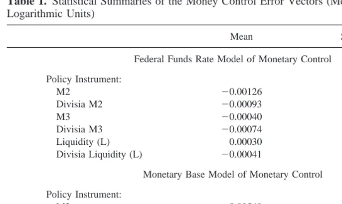
Table 1. Statistical Summaries of the Money Control Error Vectors (Measurements in Quarterly
Logarithmic Units)
Mean Standard Deviation
Federal Funds Rate Model of Monetary Control
Policy Instrument:
M2 20.00126 0.01309
Divisia M2 20.00093 0.01244
M3 20.00040 0.01246
Divisia M3 20.00074 0.01257
Liquidity (L) 0.00030 0.01103
Divisia Liquidity (L) 20.00041 0.01166
Monetary Base Model of Monetary Control
Policy Instrument:
M2 20.00540 0.0090
Divisia M2 20.00470 0.0080
M3 20.00190 0.0065
Divisia M3 20.00191 0.0066
Liquidity (L) 20.00164 0.0064
1964:Q1 and then forecasting the subsequent quarter value of the dependent variable. The forecast is subtracted from the actual value of the dependent variable to generate the first observation in the money control error vector for that policy instrument, in that model of monetary control. Equation (8) is re-estimated, forecasts are generated, and a money control error vector is computed using a rolling horizon approach until a vector of money control errors is generated for the given policy instrument over the period 1964:Q2–1997: Q4. This procedure is repeated for each policy instrument. Money control error vectors are then generated with the monetary base model of monetary control using the same procedure, but substituting equation (9) for equation (8).
The rolling horizon approach is used to produce time-varying coefficient models which model the changing relationship between the policy instrument and the federal funds rate or the changing relationship between the policy instrument and the monetary base. Potential sources of change in the relationship between the control variable and the policy instrument include changes in the level of inflation, the economy’s position in the business cycle, etc.
Means and standard deviations of the money control error vectors appear in Table 1.24 In the federal funds rate model of monetary control the mean money control errors are close to zero—ranging from20.00126 in quarterly logarithmic units for M2 (i.e., about 20.5 percent at an annualized rate) to 0.00030 in quarterly logarithmic units for Liquidity (i.e., about 0.1 percent). Standard deviations of the money control error vectors range from
24If one takes the midpoint of the M2, M3 or L targets set since the mid-1970’s and compares actual growth to targeted growth it is clear that the mean error is not zero. However, the Fed was not attempting to solely control either M2, M3 or L during this time. So, announced M2, M3 or L targets are not an adequate guide as to what is possible regarding the mean error for these particular policy instruments.
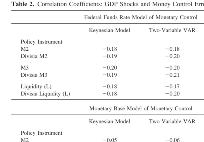
Table 2. Correlation Coefficients: GDP Shocks and Money Control Errors
Federal Funds Rate Model of Monetary Control
Keynesian Model Two-Variable VAR Four-Variable VAR
Policy Instrument
M2 20.18 20.18 20.45
Divisia M2 20.19 20.20 20.45
M3 20.20 20.20 20.45
Divisia M3 20.19 20.21 20.45
Liquidity (L) 20.18 20.17 20.44
Divisia Liquidity (L) 20.18 20.20 20.45
Monetary Base Model of Monetary Control
Keynesian Model Two-Variable VAR Four-Variable VAR
Policy Instrument
M2 20.05 20.06 20.12
Divisia M2 20.05 20.09 20.12
M3 20.03 20.04 20.08
Divisia M3 20.01 20.03 20.10
Liquidity (L) 0.05 0.02 0.01
0.01103 in quarterly logarithmic units for Liquidity (i.e., about 4.5 percent) to 0.01309 in quarterly logarithmic units for M2 (i.e., about 5.3 percent).
In the monetary base model of monetary control the absolute values of the mean money control errors are generally higher, but the standard deviations are generally smaller. The largest mean money control error is for Liquidity at20.00164 in quarterly logarithmic units (i.e., about 20.67 percent) and the smallest mean error is for M2 at20.00540 in quarterly logarithmic units (i.e., about 22.2 percent). Standard deviations range from 0.0063 in quarterly logarithmic units (i.e., about 2.5 percent) for Divisia L to 0.0090 in quarterly logarithmic units (i.e., about 3.65 percent) for M2.
Simulated error vectors generated with the federal funds rate model and monetary base model, respectively, for each of the policy instruments, are individually recycled as the money control error vector for that particular policy instrument in equation (7). Note, it is inappropriate to compute the money control error as the deviation of the actual value of a policy instrument from the rule-specified levels over the sample period. Errors computed this way would be inaccurate measures of money control error because at no time during this period was the Fed focusing explicitly on any of the proposed policy instruments as the singe instrument of monetary policy.
Separate GDP simulations are conducted with each of the three macroeconomic models, with the six respective policy instruments, and the two different models of monetary control. Table 2 displays correlation coefficients between the vectors of GDP shocks (generated by estimating each of the three macroeconomic models using each of the respective policy instruments) and the money control error vectors computed using the federal funds rate or monetary base model of money control. Correlations obtained between GDP shocks and money control errors generated by the federal funds rate model of monetary control are negative and not unsubstantial, with the largest negative corre-lations occurring in the four-variable VAR model.25Correlations obtained between GDP shocks and money control errors generated by the monetary base model are mostly negative, but generally close to zero.
A strategy of using a monetary variable to target nominal GDP, may perform better than a strategy of using a control variable (e.g., the Federal Funds rate or the monetary base) to directly target nominal GDP—if shocks to the linkage between the control variable and policy instrument are negatively correlated with the shocks between the policy instrument and nominal GDP. Negative correlations, as seen under the federal funds rate model of monetary control, suggest that positive GDP shocks will often be partially offset by negative money control errors and vice-versa, thus improving the level of price stability obtainable by the adaptive policy rule. The larger negative correlations between GDP shocks and money control errors, combined with the lower mean money control errors in the federal funds rate model, would seem to suggest that for the policy instruments examined, the federal funds rate is a preferable control variable to the monetary base.
Given one specific model of monetary control (i.e., either the federal funds rate model or the monetary base model) and one specific macroeconomic model, the correlation coefficients tend to be fairly similar in size for all six policy instruments. Consequently, differences in rule performance that arise between the different policy instruments (within
a single macroeconomic model and model of monetary control) are unlikely to result from differences in the interactions between GDP shocks and money control errors.
The RMSEs resulting from the GDP simulations appear in Table 3. It is apparent from these results that all of the policy rules meet the six criteria for rule success. First, consider
Figure 1. GDP growth path: Divisia L rule in a four-variable VAR (Federal Funds Rate Model of
Monetary Control).
Table 3. GDP RMSEs (l50.25 and 4-year Moving Average Velocity Growth Rate)
Historical GDP RMSE:
From a 3 percent growth path: 1.0209
From a 7.46 percent* growth path: 0.1663
Federal Funds Rate Model of Monetary Control
Keynesian Model Two-Variable VAR Four-Variable VAR
Policy Instrument
M2 0.0350 0.0277 0.0287
Divisia M2 0.0304 0.0247 0.0275
M3 0.0437 0.0299 0.0325
Divisia M3 0.0370 0.0272 0.0328
Liquidity (L) 0.0411 0.0277 0.0303
Divisia Liquidity (L) 0.0295 0.0245 0.0288
Monetary Base Model of Monetary Control
Keynesian Model Two-Variable VAR Four-Variable VAR
Policy Instrument
M2 0.0474 0.0386 0.0407
Divisia M2 0.0432 0.0361 0.0405
M3 0.0492 0.0287 0.0338
Divisia M3 0.0399 0.0270 0.0345
Liquidity (L) 0.0431 0.0258 0.0311
Divisia Liquidity (L) 0.0313 0.0245 0.0308
simulated rule performance in comparison to the performance of actual discretionary monetary policy. The RMSE of the historical nominal GDP time path from the non-inflationary time path is 1.0209. All of the monetary rules, in three different economic models, deliver substantially higher levels of long-run price stability (as measured by lower RMSEs) than historical, discretionary monetary policy—satisfying one criterion for rule success.
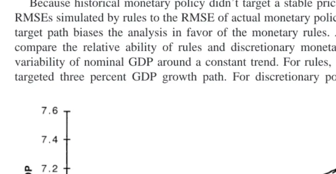
Because historical monetary policy didn’t target a stable price level, a comparison of RMSEs simulated by rules to the RMSE of actual monetary policy from the three percent target path biases the analysis in favor of the monetary rules. Alternatively, one could compare the relative ability of rules and discretionary monetary policy to reduce the variability of nominal GDP around a constant trend. For rules, the constant trend is the targeted three percent GDP growth path. For discretionary policy, the constant trend Figure 2. GDP growth path: Divisia M3 rule in a four-variable VAR (Federal Funds Rate Model
of Monetary Control).
Figure 3. GDP growth path: Divisia M2 rule in a four-variable VAR (Federal Funds Rate Model
utilized is the historical, 7.6 percent average rate of nominal GDP growth over the 1964:Q2—1997:Q4 sample.
The RMSE of actual, nominal GDP around the historical trend is 0.1663. Using this value as a benchmark, it is clear that all of the policy rules substantially reduce the variability of nominal GDP about a fixed trend—relative to historical monetary policy.
When accounting for financial innovations and changing structural relationships be-tween macroeconomic variables through GDP shocks and money control errors of likely magnitudes, all of the policy rules perform well— delivering a relatively high degree of price stability. The RMSEs of simulated GDP from the non-inflationary time path fall within a narrow range—from a low of 0.0245 for Divisia L in the two-variable VAR to a high of 0.0492 for M3 in the Keynesian model (with the monetary base used as the control variable). Figures 1–3 further illustrate the performance of the three Divisia measures of money in the four-variable VAR model. Note, for each policy instrument and respective policy rule, simulated GDP never strays very far from the non-inflationary GDP target time path.
Thus, one could conclude that over the sample period all of the policy instruments exhibited a strong and stable enough relationship with nominal GDP to have performed well in McCallum’s rule. This conclusion would probably hold in the future. The period examined in this study, 1964 –1997, is one characterized by many changes in structural relationships between macroeconomic variables, much financial innovation and various large random shocks to the relationships between the control variable and the policy instrument as well as the relationships between the policy instruments and goal variable. Regarding the effects on rule performance of financial innovations and other sources of changing structural relationships between a measure of money and GDP, consider the following example. Suppose a structural change occurs in the relationship between a policy instrument in McCallum’s Rule and nominal GDP causing the income velocity of the policy instrument to rise. At the point in time where this change begins to manifest itself, the GDP shocks in the constant-coefficient macro models used here increase in size. This pushes simulated GDP away from the GDP target. In response to increasing velocity, the four-year moving average velocity growth rate in McCallum’s rule gradually rises. This reduces the growth rate of the policy instrument which then reduces deviations of nominal GDP from the target path. The feedback term in equation (1) provides an even more immediate monetary policy response to the changing velocity growth rate.
The responses of the second and third terms on the right side of equation 1, make it unnecessary for a policy instrument to maintain an absolutely stable relationship with GDP, in order for the rule to successfully keep GDP close to the target. Although there is some degree of velocity instability that would eradicate the success of any policy instrument and corresponding version of McCallum’s rule, changing structural relation-ships between the policy instruments examined here and GDP didn’t cross that threshold during the last three decades. Design features added purposefully by McCallum to make the rule fully operational adjust the growth rate of the policy instrument automatically to accommodate changes in velocity resulting from; structural changes in the economy or transient random shocks.
VAR model, with either model of monetary control), a Divisia measure of money tends to produce a smaller RMSE than its monetary aggregate counterpart. However, the difference is usually not substantial—and never larger than 0.012. These results suggest that for the broader levels of monetary aggregation (i.e., M2 and above), the performance of McCallum’s Rule is robust for measures of money computed through unweighted summation of the component assets or through the measurement of monetary services that are obtained with Divisia monetary indexes.
Compared to the other policy instruments, Divisia L produces the lowest RMSEs in all but the four-variable VAR with the federal funds rate model of monetary control. However, the performance of Divisia L as a policy instrument is generally not overwhelm-ingly superior to the other Divisia measures of money examined here. This contrasts with GDP simulations conducted over the same sample period and with the same economic models in Thornton (1999). In that study policy rules were evaluated that used narrower measures of money as their policy instruments. Thornton (1999) found that Divisia M2 versions of McCallum’s rule performed much better than Divisia M1 or Divisia M1A versions of McCallum’s Rule. Thus, it seems that in the case of the broad Divisia measures of money, while the level of aggregation matters, it doesn’t seem to matter very much above the M2 level.
Comparing simulation results across the 2 models of monetary control, it appears that with the exceptions of M3, Divisia M3 and L in the two-variable VAR model, the federal funds rate model permits a slightly higher degree of price stability (i.e., a lower RMSE) than the monetary base model of monetary control. The generally better performance of the federal funds rate as a control variable generally results from two factors; (1) smaller mean money control errors, and (2) larger negative correlations between the money control error and the GDP shocks. Although the standard deviations of the money control error are smaller in the monetary base model of money control, this is less of an advantage than a smaller mean error because the feedback properties of McCallum’s rule permit much of the standard deviation in money growth caused by these errors to be offset.
Simulation results suggest that the Fed could successfully use an M2, Divisia M2, M3, Divisia M3, L or, Divisia L rule to maintain much greater levels of price stability and much lower levels of GDP variability than has been achieved under discretionary mon-etary policy— even in an environment characterized by random shocks and changing structural relations among key macroeconomic variables. However, operationalizing the L or Divisia L rules could be somewhat more problematic than operationalizing rules that use M2, Divisia M2, M3 or Divisia M3 as policy instruments. This is in part because data on L and Divisia L are no longer published by the FED in the H.6 release, making compliance with a L or Divisia L rule more difficult for the public to monitor. Moreover, data on L and Divisia L traditionally have been available to FED policy makers with a longer lag than data on narrower measures of money such as M2, Divisia M2, M3, or Divisia M3. This lag could also cause greater difficulties in operationalizing an L or Divisia L rule.
IV. Assessing the Policy Implications of the GDP Simulations
Conclusions regarding the ability of rules examined here to increase price stability and lower the variability of nominal GDP around a constant trend are subject to caveats. For example, suppose adoption of a policy rule alters the structural relationship between a policy instrument and the nominal GDP target. Or suppose adoption of the rule alters the structural relationship between the control variable and the policy instrument. Presumably either of these changes would reduce the effectiveness of the policy rule. In either case the design of McCallum’s rule is such that as long as the adoption of one of the versions of
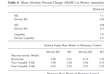
Table 4. Mean Absolute Percent Change (MAPC) in Money (annualized rates of change)
Historical Norm
M2 7.11
Divisia M2 6.08
M3 8.00
Divisia M3 6.53
Liquidity 7.81
Divisia Liquidity 6.34
Federal Funds Rate Model of Monetary Control
Divisia M2 M2 Divisia M3 M3 Divisia L L Macroeconomic Model:
Keynesian 4.60 4.41 6.14 7.39 4.99 6.78
Two-Variable VAR 3.96 4.20 5.06 5.15 4.59 4.80
Four-Variable VAR 4.92 5.55 5.55 5.35 5.08 5.14
Monetary Base Model of Monetary Control
Divisia M2 M2 Divisia M3 M3 Divisia L L Macroeconomic Model:
Keynesian 4.70 3.84 5.59 7.25 4.29 6.40
Two-Variable VAR 3.71 3.36 4.05 4.01 3.73 3.95
Four-Variable VAR 5.13 5.61 4.86 4.65 4.37 4.34
Table 5. Mean Absolute Percent Change (MAPC) in Real GDP (annualized rates of change)
Historical Norm: 3.94
Federal Funds Rate Model of Monetary Control
Divisia M2 M2 Divisia M3 M3 Divisia L L Macroeconomic Model:
Keynesian 4.15 4.25 4.23 4.34 4.14 4.40
Four-Variable VAR 3.51 3.34 3.79 3.55 3.80 3.55
Monetary Base Model of Monetary Control
Divisia M2 M2 Divisia M3 M3 Divisia L L Macroeconomic Model:
Keynesian 4.44 4.50 4.22 4.33 4.19 4.44
McCallum’s Rule (evaluated above) doesn’t eliminate or excessively weaken the structural relationship between the policy instrument and GDP, the rule will automatically make the modifications necessary to accommodate either type of a structural change through adjustments in the velocity and feedback terms.
Another criticism is that policy rules targeting levels of nominal income will produce greater variability in the policy instrument and thus real output than has been experienced historically. This hypothesis can be evaluated using results presented in Tables 4 and 5. Using the mean absolute percent change (MAPC) in the policy instrument as a measure of variability, during 1964:Q2–1997:Q4, the actual quarterly MAPCs in the policy instruments ranged from 6.08 percent for Divisia M2 to 8.0 percent for M3, respectively (at annualized rates). Table 4 shows that in all three economic models and both models of monetary control, all six of the policy instruments would have been considerably less variable under the rule specified by equation 1.
The likely variability of real GDP, resulting from the adoption of one of the policy rules examined here, can only be evaluated in the Keynesian and four-variable VAR. The historical MAPC of real GDP, during 1964:Q2–1997:Q4, was 3.94 percent (at annualized rates). The MAPCs of real GDP obtained in the four-variable VAR, under all of the policy rules, are slightly below the historical norm. In the Keynesian model, the MAPCs of real GDP in all of the policy rules are just slightly above the historical norm— but never by much more than 0.5 percent. These results indicate that the benefits of price stability are not likely to be obtained at the costs of substantially increased instability in the policy instrument and/or in real output. Presumably then, the costs of targeting a stable price level, are unlikely to be as large as some have suggested—further strengthening arguments for the adoption of an adaptive rule that targets levels of GDP to produce long-run price stability.
One final caveat addresses problems caused by GDP data revision. Given the length of time over which revisions are made and the sometimes substantial size of those revisions, the policy maker implementing a version of McCallum’s rule specified by equation (1) is probably reacting to incorrect (initial) estimates of GDP. The Bureau of Economic Analysis (BEA) estimates that nine-tenths of the revisions from the preliminary estimate of the quarterly percent change in GDP to the final estimate range from 21.2 to 1.4 percent (at an annualized rate). Thus, if the preliminary estimate of the 1999:Q4 change in GDP was 3.0 percent, during the next 2 months it is likely to be revised down to as low as 1.8 percent or revised up as high as 4.4 percent. The long-run revisions are larger. Nine-tenths of the revisions from the preliminary estimate to the latest estimate range from 22.1 to 2.7 percent.26
Orphanides (1998) examined the impact of the GDP data revision problem on the performance of Taylor’s rule which uses the federal funds rate to target GDP. He found that GDP data revisions would have produced substantial changes in the policy recom-mendations of Taylor’s rule— changes so large they exceeded the standard deviation of the historical quarterly change in the federal funds rate during the 1987–1992 sample period. Theoretically, because the GDP simulations conducted in Section III ignore the
data revision problem, they could be substantially overstating the likely performance of the versions of McCallum’s rule that are being evaluated.
One approach utilized to assess the impacts of this informational problem assumes that policy makers could wait an additional quarter, to obtain a more accurate estimate of nominal GDP, before responding to deviations of GDP from the non-inflationary target path. In this case policy makers might utilize the rule in equation (10).
DRMt50.007392~1/16!~Xt212Xt2172Mt211Mt217!1l@X*t222Xt22# (10)
In this version of the rule the feedback term is based on the deviation of nominal GDP from the target path—two quarters past. So, for example, a policy maker calculating, on April 1, the rule-prescribed change in the policy instrument for the second quarter of a given year would compare BEA’s final GDP estimate of fourth quarter GDP (Xt22) to the fourth quarter GDP target (X*t22). GDP simulations were conducted over the sample 1964:Q2–1997:Q4 using the three macroeconomic models, and equation (10), with Divisia L as the policy instrument.27Results from these simulations appear in Table 6.
Another approach for assessing the impacts of the informational problem caused by GDP revisions is to directly incorporate the effects of GDP revision error into the simulations. This is done by defining BEA’s ultimate, long-run, revised calculation28of the value of nominal GDP in time t2 1 as Xt21 and letting Xtp21 be the preliminary estimate of prior quarter GDP, reported by the BEA. The relationship between BEA’s ultimate, long-run, revised calculation of GDP and the preliminary estimate is: Xt215
27Simulation results using the rules specified by equations 10 and 12 and with either M2 or Divisia M2 as the policy instrument appear in Thornton (1999). Results show that the problems associated with GDP data revisions have an inconsequential effect on the performance of M2 or Divisia M2 rules. Divisia L was selected as the policy instrument in the simulations in the current study in order to examine the effects of the GDP data revision problem on another potential policy instrument and because of the Divisia L rule’s excellent perfor-mance in GDP simulations conducted in Section 3.
28This corresponds to the ex post GDP time series data.
Table 6. Effects of GDP Data Revisions on the Performance of McCallum’s Rule (Federal
Funds Rate Model of Monetary Control)
GDP RMSEs
Keynesian Model Two-Variable VAR Four-Variable VAR Lagged Policy
Response Version of McCallum’s Rule 0.03539 0.02693 0.03442
McCallum’s Rule
Directly Incorporating Effects of GDP Revision Errors
0.03002 0.02492 0.02912
MAPCs of Divisia L (annualized rates of change)
Keynesian Model Two-Variable VAR Four-Variable VAR Lagged Policy
Response Version of McCallum’s Rule 5.45 4.68 5.59
McCallum’s Rule
Directly Incorporating Effects of GDP Revision Errors
Xtp211 REt21. The final revision error (RE) is expressed in quarterly logarithmic units. If a policy maker wanted to respond in the current quarter to last quarter’s missed GDP target level, using BEA’s preliminary estimate of last quarter’s GDP, the policy rule would be;
DRMt50.007392~1/16!~Xt212Xt2172Mt211Mt217!1l@X*t212Xt21
p #
(11)
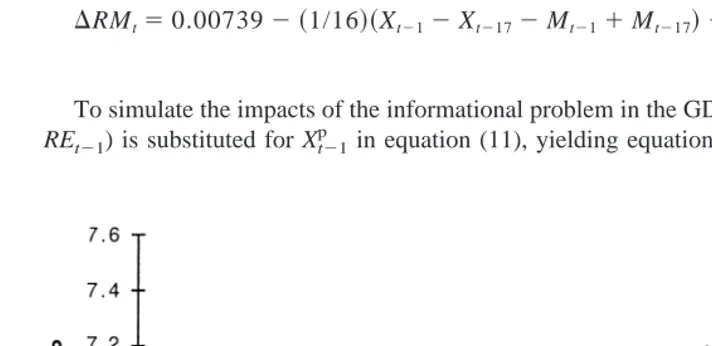
To simulate the impacts of the informational problem in the GDP simulations, (Xt212 REt21) is substituted for Xt21
p
in equation (11), yielding equation 12.
Figure 4. GDP growth path: Divisia L rule in a four-variable VAR that incorporates GDP revision
error (Federal Funds Rate Model of Monetary Control).
Figure 5. GDP growth path: Divisia L rule with a two-Quarters lagged policy response in a
DRMt50.007392~1/16!~Xt212Xt2172Mt211Mt217!1l@X*t212~Xt21 2REt21!# (12) A vector of revision errors is generated for the entire sample. This vector of revision errors is of the magnitude reported by the BEA for its preliminary to its last, annually revised GDP estimate. Simulations are conducted with; (1) the revision error vector incorporated into equation 12, (2) each of the three macroeconomic models, and (3) Divisia L as the policy instrument. The RMSEs of simulated GDP from the non-inflationary target path and the MAPCs of the policy instrument are reported in Table 6 (assuming the federal funds rate model of monetary control).
When comparing GDP RMSEs in Table 6 to GDP RMSEs in Table 3 it is apparent that both; (1) incorporating revision error into the GDP simulations, and (2) utilizing a rule with a longer response time have inconsequential impacts on the ability of the Divisia L rule to produce a high degree of price stability! In both cases, the RMSEs of simulated GDP from the target path increase only slightly. Why? When a policy instrument exhibits a strong relationship with GDP, even sizable GDP data revisions that push simulated GDP away from the target path can be easily mitigated by subsequent changes in rule-prescribed money growth.29Utilization of policy rules based on a feedback term with a two-quarter lag, lengthen the response time of monetary policy to shocks that would drive GDP away from the target path increasing the GDP RMSE slightly more. But again, the strong relationship between the policy instrument and GDP permit the rule to perform well— even with the longer response time.
Orphanides (1998) reports that incorporating the impacts of GDP revision errors produces substantially larger changes in the policy instrument (i.e., the federal funds rate) in Taylor’s rule. In contrast, the Divisia L version of McCallum’s rule still produces a scenario in which the policy instrument is less variable than it was historically. Moreover, the increase in the MAPCs over the GDP simulations where the impacts of GDP data revisions are not considered (i.e., as reported in Table 4) is small—ranging from 0.06% in the Keynesian model to 0.51% in the four-variable VAR (at an annualized rate).
Figures 4 and 5 illustrate the impacts of the informational problem on the simulated GDP time paths. As both figures illustrate the deviations of nominal GDP from the targeted time path remain quite small. Thus, in contrast to results obtained by Orphanides (1998) for Taylor’s rule, this study finds that a Divisia L version of McCallum’s rule continues to perform quite well— even when incorporating the difficulties policymakers would face as a result of GDP data revisions.
V. Conclusion
The performance of six different policy instruments is assessed using variations of McCallum’s adaptive rule for targeting levels of nominal GDP. Three economic models are used, respectively, to examine rule performance by simulating values of nominal GDP during 1964:Q2–1997:Q4. Rule performance is measured primarily by the RMSE of
simulated GDP from the non-inflationary target path and secondarily by the variability of the policy instrument and real GDP—relative to historical norms.
Rules utilizing any one of the six policy instruments appear to meet all six criteria for a successful policy rule. Moreover, all the rules examined here are operational and central bank compliance could be monitored using one of the methods explained in Section II. Unlike rules using narrower measures of money or interest rates, all of the rules examined here perform well in a variety of plausible macroeconomic models—including one that incorporates an interest rate. Rules utilizing the broader monetary aggregates or broader Divisia measures of money as policy instruments perform well when; (1) financial innovations, regulatory changes or shocks alter the linkages between the policy instrument and the intermediate target, (2) financial innovations, regulatory changes or shocks alter the linkages between the control variable and the policy instrument, (3) policy makers cannot precisely control the policy instrument over periods of time as short as one quarter, and (4) policy makers cannot use the most accurate calculation of prior quarter GDP to determine current quarter money growth.
The rules examined here also outperform historical discretionary policy in promoting long-run price stability and lowering the variability of nominal GDP around a constant trend. The feedback properties of the different versions of McCallum’s rule, combined with the relative strength and stability of the relationship between the respective policy instruments and the GDP target, are responsible for the rules’ excellent performance.
GDP simulation results do suggest that the method of monetary aggregation generally affects rule performance. Rules using Divisia measures of money as their policy instru-ment usually deliver greater amounts of long-run price stability than rules using their monetary aggregate counterparts. However, the method of aggregation doesn’t seem to matter very much. Finally, while the choice of control variable (i.e., the federal funds rate or the monetary base) doesn’t appear to have a critical impact on rule success, some improvement in rule performance is gained by using the federal funds rate to target the rule-specified growth rate in the policy instrument.
These results strengthen the case for the adoption of an adaptive rule to be used in the formulation of monetary policy— or at a minimum, to provide information useful in the formulation of discretionary monetary policy.
Extraordinarily helpful comments were received from Bennett McCallum, Allan H. Meltzer, Michael Belongia, and an anonymous referee. Any errors are the sole responsibility of the author.
References
Aiyagari, S. R. Summer 1990. Deflating the case for zero inflation. Federal Reserve Bank of Minneapolis Quarterly Review 14:2–11.
Anderson, R. G., Jones, B. E., and Nesmith, T. D. January/February 1997a. Introduction to the St. Louis monetary services index project. St. Louis Federal Reserve Bank Review 79:25–29. Anderson, R. G., Jones, B. E., and Nesmith, T. D. January/February 1997b. Monetary aggregation
theory and statistical index numbers. St. Louis Federal Reserve Bank Review 79:31–51. Anderson, R. G., Jones, B. E., and Nesmith, T. D. January/February 1997c. Building new monetary
Barnett, W. A. 1980. Economic Monetary Aggregates: An application of index number and aggregation theory. Journal of Econometrics 14:11–48.
Barnett, W. A. 1987. The microeconomic theory of monetary aggregation. New Approaches to Monetary Economics: Proceedings of the Second International Symposium in Economic Theory and Econometrics. International Symposia in Economic Theory and Econometrics Series. Cambridge: Cambridge University Press, pp. 115–168.
Barnett, W. A. Summer 1990. Developments in monetary aggregation theory. Journal of Policy Modeling 12:205–257.
Barnett, W. A., Fisher, D., and Serletis, A. 1992. Consumer theory and the demand for money. Journal of Economic Literature 30:2086–2119.
Barnett, W. A., Hinich, M., and Yue, P. 1991. Monitoring monetary aggregates under risk aversion. Monetary Policy on the 75th Anniversary of the Federal Reserve System (M. Belongia, ed.). Boston: Kluwer Academic Publishers, pp. 189–222.
Barnett, W. A., Offenbacher, E., and Spindt, P. 1984. The new divisia monetary aggregates. Journal of Political Economy 92:1049–1085.
Barnett, W. A., and Spindt, P. 1982. Divisia monetary aggregates: Compilation, data, and historical behavior. Federal Reserve Bulletin 68:291–299.
Batten, D. S., and Thornton, D. L. June/July 1985. Are weighted monetary aggregates better than simple-sum M1? St. Louis Federal Reserve Bank Review 67:29–40.
Becketti, S., and Morris, C. Fourth Quarter 1992. Does money still forecast economic activity? Federal Reserve Bank of Kansas City Economic Review 77:65–77.
Belongia, M. October 1996. Measurement matters. Journal of Political Economy 104:1065–1083. Belongia, M., and Batten, D. S. 1992. Selecting an intermediate target variable for monetary policy when the goal is price stability. Working Paper No. 92-008A. St. Louis Federal Reserve Bank. Bureau of Economic Analysis. Friday, July 31, 1998. National Income and Products Accounts,
Second Quarter 1998 GDP, Revised Estimates. BEA News Release.
Clark, T. E. Third Quarter 1994. Nominal GDP targeting rules: Can they stabilize the economy? Federal Reserve Bank of Kansas City Economic Review 79:11–25.
Dueker, M. January/February 1995. Narrow vs. broad measures of money as intermediate targets: Some forecast results. St. Louis Federal Reserve Bank Review 77:41–51.
Dotsey, M., and Otrok, C. Winter 1994. M2 and monetary policy: A critical review of the recent debate. Federal Reserve Bank of Richmond Economic Quarterly 80:41–59.
Engle, R., and Granger, C. W. March 1987. Co-integration and error correction: Representation, estimation, and testing. Econometrica 55:251–276.
Engle, R., and Yoo, B. 1987. Forecasting and testing in co-integrated systems. Journal of Econo-metrics 35:143–159.
Fair, R. C. and Howrey, E. P. 1996. Evaluating alternative monetary policy rules. Journal of Monetary Economics 38:173–194.
Farr, H. T., and Johnson, D. May 1985. Revisions in the Monetary Services (Divisia) Indexes of Monetary Aggregates. Board of Governors of the Federal Reserve System Special Studies Paper, No. 189.
Feldstein, M., and Stock, J. H. 1993. The use of a monetary aggregate to target nominal GDP. NBER Working Paper No. 4304.
Friedman, B. 1988. Conducting monetary policy by controlling currency plus noise: A comment. Carnegie-Rochester Conference Series on Public Policy 29:205–12.
Friedman, B., and Kuttner, K. K. June 1992. Money, income, prices and interest rates. American Economic Review 82:472–492.
Eco-nomics Discussion Series, Operating Procedures and the Conduct of Monetary Policy: Confer-ence Proceedings. (M. Goodfriend and D. H. Small, eds.).
Jefferson, P. N. 1997. ‘Home’ Base and Monetary Base Rules: Elementary Evidence from the 1980s and 1990s. Federal Reserve Board. Finance and Economics Discussion Series, 1997-21. Judd, J. P., and Motley, B. Summer 1991. Nominal feedback rules for monetary policy. Federal
Reserve Bank of San Francisco Economic Review 2:3–17.
Judd, J. P., and Motley, B. Fall 1992. Controlling inflation with an Interest Rate Instrument. Federal Reserve Bank of San Francisco Economic Review 3:3–22.
Judd, J. P., and Motley, B. Fall 1993. Using a nominal GDP rule to guide discretionary monetary policy. Federal Reserve Bank of San Francisco Economic Review 4:3–11.
Marty, A., and Thornton, D. July/August 1995. Is There a Case for ‘Moderate’ Inflation? Federal Reserve Bank of St. Louis Review 77:27–37.
McCallum, B. September/October 1987. The case for rules in the conduct of monetary policy: A concrete example. Federal Reserve Bank of Richmond Economic Review 73:10–18.
McCallum, B. 1988. Robustness properties of a rule for monetary policy. Carnegie-Rochester Conference Series on Public Policy 29:173–203.
McCallum, B. August 1990. Could a monetary base rule have prevented the Great Depression? Journal of Monetary Economics 26:3–26.
McCallum, B. 1993. Specification and analysis of a monetary policy rule for Japan. Bank of Japan Monetary and Economic Studies 11:1–45.
McCallum, B. 1998. Issues in the design of monetary policy rules. Handbook of Macroeconomics (J. B. Taylor and M. Woodford, eds.). North Holland.
Orphanides, A. 1998. Monetary Policy Rules Based on Real Time Data. Finance and Economics Discussion Series 1998-3.
Petersen, D. J. November/December 1995. FYI—Monetary aggregates, payments technology and institutional factors. Federal Reserve Bank of Atlanta Economic Review 80:30–37.
Rasche, R. 1995. Pitfalls in counterfactual analyses of policy rules. Open Economies Review 6:199–202.
Rottemberg, J. J. 1991. Monitoring Monetary Aggregates Under Risk Aversion. Monetary Policy on the 75th Anniversary of the Federal Reserve System (M. Belongia, ed.). Boston: Kluwer Academic Publishers, pp. 189–222.
Rottemberg, J. J., Driscoll, J., and Porteba, J. M. January 1995. Money, output, and prices: Evidence from a new monetary aggregate. Journal of Business and Economic Statistics 13:67–83. Taylor, J. B. 1993. Discretion versus policy rules in practice. Carnegie-Rochester Conference Series
on Public Policy 39:195–214.
Thornton, D. March/April 1996. The costs and benefits of price stability: An assessment of Howitt’s rule. Federal Reserve Bank of St. Louis Review 78:23–38.
Thornton, D., and Yue, P. November/December 1992. An extended series of Divisia monetary aggregates. Federal Reserve Bank of St. Louis Review 74:35–45.
Thornton, S. September/October 1993. Can forecast-based monetary policy be more successful than a rule? Journal of Economics and Business 45:231–245.
Thornton, S. July/August 1998. Identifying a suitable policy instrument in an adaptive monetary policy rule. Journal of Economics and Business 50:379–398.