www.elsevier.com / locate / econbase
Measuring the performance of foreign direct investment:
a case study of China
*
Yanrui Wu
Department of Economics, University of Western Australia, Nedlands, WA 6907, Australia
Received 2 March 1998; received in revised form 22 January 1999; accepted 15 September 1999
Abstract
Within the new growth framework, this paper attempts to investigate the performance of foreign direct investment, i.e. how efficient FDI as one of the factor inputs in an economy has been utilised. In the empirical analyses, an input-oriented distance function approach is employed to estimate the technical efficiency of FDI in China’s coastal regions over the period 1983–1995. 2000 Elsevier Science S.A. All rights reserved.
Keywords: Input distance function; Technical efficiency
JEL classification: C24; O53
1. Introduction
Within the new growth framework, foreign direct investment (FDI) is treated as one of the factor inputs along with labour and (domestic) capital. It is argued that FDI is one of the main forces driving economic growth in the less developed countries. In particular, it has long been recognised that FDI is a major source of technology and know-how for developing countries (Balasubramanyan et al., 1996). FDI distinguishes itself from other forms of investment by its ability to transfer not only production know-how but also other technical, managerial and marketing skills. It also brings into the host countries tremendous externalities, namely, promotion of competition, and technical progress through investment in R&D, and through specialisation.
However, the experience of the developed economies shows that whether foreign capital is productive depends on some initial conditions in the hosting economies. It is particularly argued that the Marshall Plan worked for Europe after the Second World War because the European countries receiving aid possessed the necessary structural, institutional and attitudinal conditions, e.g.
well-*Tel.:161-8-9380-3964; fax: 161-8-9380-1016. E-mail address: [email protected] (Y. Wu)
integrated commodity and money markets, highly developed transport facilities, a well-trained and educated workforce, and an efficient government bureaucracy. These preconditions helped convert new capital effectively into a higher level of output in Europe.
Since the inception of economic reform in 1978, China has experienced almost two decades of rapid growth of foreign direct investment. This growth was particularly impressive in the first half of the 1990s. As a result, FDI as a share of total investment has increased rapidly during the past 15 years. Immediately, one may ask how efficient FDI has been utilised in the Chinese economy, given the poor infrastructure and an economic system in transition. The current paper presents a preliminary analysis on this issue. In particular, it focuses on comparing FDI performance among the Chinese regions. The next section deals with the conceptual issues about performance measurement. This is followed by empirical estimations and interpretations of the results. Finally, some summary remarks are presented in the conclusion.
2. Measuring FDI performance: an input distance function approach
Following the new growth theory, FDI is assumed to be a factor input and its performance can then be examined in the framework of production functions. Various methods have so far been developed to measure the performance of factor inputs. The approach employed in this study falls into the broad category of the stochastic frontier method which is related to the concept of input-oriented technical
1
efficiency proposed by Farrell (1957). The important difference between the traditional production function method and the production frontier technique is that the latter allows for production above the cost frontier given outputs or below the best practice output given inputs. Then, the ratio of the actual input used (observed output) over the minimal input requirement (potential output) gives an indicator of the performance of the factor input considered.
According to Shephard (1953) an input distance function can be defined as follows
D(Y, X )5maxhu: X /u[L(Y )j (1)
where L(Y ) is the input requirement set, i.e.
L(Y )5hX: X can produce Yj (2)
and Y is the output vector which can be produced using input vector X. The distance function, D(Y,
X ), is non-decreasing, positively linearly homogenous and concave in X, and non-increasing in Y
¨
(Fare and Grosskopf, 1990; Lovell et al., 1991). ¨
Following Fare and Primont (1995, p. 20), the input distance function is illustrated in Fig. 1, where the input set, L(Y ), corresponds to a given output Y . Given an input vector X , the value of D(Y , X )0 0 0 0 0
¨ puts X /D(Y , X ) on the boundary of L(Y ) and on the ray through X . According to Fare and0 0 0 0 0 Grosskopf (1996, p. 51), X[L(Y ) if and only if D(Y, X )$1, which implies that the distance function will take a value which is greater than or equal to unity, depending on whether the input vector, X, is located above or on the inner boundary of the input set. Thus, the input distance function seeks the greatest possible radial shrinkage of observed input bundle X which still allows production of
1
Fig. 1. Input set and distance function.
observed output bundle Y. It gives an indicator of factor performance by comparing the largest feasible contraction of an input with the observed use of the input.
Consider a Cobb–Douglas functional form, the statistical formulation of the input distance function 2
defined in Eqs. (1) and (2) can be expressed as
v
D(Y, X )5f(X, Y,r)e (3)
where r is a vector of parameters to be estimated and v is the random disturbance term intended to capture the effects of measurement error and statistical noise and is assumed to be independently and
2
identically distributed as N(0, sv). The basic problem with the estimation of Eq. (3) is that the left-hand side of the distance function, D(Y, X ), is not observable. Furthermore, if production occurs on the frontier, the distance function has a value of unity and hence the dependent variable is invariant. In logarithmic form, the left-hand side of the distance function will be zero for all observations (i.e. ln D(Y, X )5ln 150). However, this problem can be avoided when the property that
¨
the distance function is homogeneous of degree one in inputs is imposed (Fare and Primont, 1995). That is,
D(Y,kX )5kD(Y, X ) (4)
Thus, if one of the inputs such as X is chosen and assume0 k51 /X , then0
D(Y, X /X )0 5D(Y, X ) /X0 (5)
For the logarithmic form, Eq. (5) can be converted into
2
ln (D(Y, X ) /X )5ln D(Y, X /X )5ln f(Y, X /X )1v (6)
0 0 0
That is,
2ln (X )5ln f(Y, X /X )1v2ln D(Y, X ) (7)
0 0
Replace the unobservable ln D(Y, X ) by u in Eq. (7) to obtain a stochastic input distance function
2ln(X )5ln f(Y, X /X )1v2u (8)
0 0
2 where u is non-negative and assumed to have a normal distribution with zero mean and variancesu. Based on the conditional distribution of u given´5v2u, the input distances would be predicted as
u
D5E[e u´] (9)
Technical efficiency can then be estimated using the property that the distance function is the reciprocal of the Farrell input-oriented measure of technical efficiency. Eqs. (8) and (9) can be estimated using the maximum likelihood method (Coelli and Perelman, 1996).
3. Empirical estimation and results
In the empirical model, the production process is assumed to involve one output and three inputs. The inputs are labour (L ), domestic (K ) and foreign (FDI) capital stocks. The causal relationship
3
between output and foreign investment has been well documented in the literature. In this study it is assumed that there is one-way causality from FDI to output. Thus, the implied relationship is that GDP is a function of labour, and domestic and foreign capital stocks. For the purpose of empirical
4 estimation, assume a Cobb–Douglas function form for the input distance function D(?), that is,
ln(D )5a 1a ln(L )1b ln(K )1hln(FDI)1g ln(GDP)1v2u (10)
0 l k
where GDP takes the value of gross domestic product, v and u are defined as in Eq. (8) and
al1bk1h51 (11)
which ensures the homogeneity of the distance function in inputs. Substituting Eq. (11) into Eq. (10) leads to the following form
ln(D )2ln(FDI )5a01alln(L / FDI)1bkln(K / FDI)1g ln(GDP)1v2u (12)
Since the frontier of technology is estimated, the input distance function D(?) equals one and thus the left-hand side of Eq. (12) becomes 2ln(FDI). As a result, the final model estimated is the reduced form of Eq. (12), that is:
3
For literature surveys, readers may refer to Krueger (1987), Karikari (1992) and Shan et al. (1999). 4
2ln(FDI)5a 1a ln(L / FDI)1b ln(K / FDI)1g ln(GDP)1v2u (13)
0 l k
It is clear that Eq. (13) is equivalent to the general form Eq. (8) replacing X by foreign capital stock.0 It is also assumed that
u5d01d1t1√ (14)
2 where√ is defined by the truncation of the normal distribution with zero mean and variancesu such that the point of truncation is (2d02d1t), that is,√$ 2d02d1t, and, thus, the u’s are non-negative
2 and obtained by truncation at zero of the normal distribution with mean (d01d1t) and variances,su. The inclusion of a time trend is to catch the variation in the performance of FDI over time. A main
5
problem with estimating Eqs. (13) and (14) is the possible presence of endogeneity. To overcome this problem, instrumental variables are employed to estimate GDP. However, the choice of instrumental variables is limited due to the data requirement (for all regions over the entire period considered). In the final estimation, following Grosskopf and Hayes (1993), the logarithm of GDP is regressed on the reciprocal of the logarithm of population, one over the square root of population and the capital–
6 labour ratio in the regions.
The above empirical specification described is applied to a data sample covering China’s 10 coastal 7
regions. The statistics are drawn from various issues of China’s Statistical Yearbook. Employment is represented by the total number of labour employed instead of man-hours due to the lack of data on the latter. Both domestic and foreign capital stocks are estimated by assuming a rate of depreciation of 5%, and using the following structure of capital formation
Kt5(12g)Kt211It (15)
where g is the rate of depreciation, and I is the investment in year t.t
8
Foreign capital stock is estimated by assuming that 1978 foreign capital was zero. The data of net domestic capital stock are estimated from gross investment data in each year. For this purpose, the capital stock in the first period is assumed to be the sum of all past investments and a rate of 5% is allowed for capital depreciation. Symbolically,
where It5I e , and0 u and I0 are estimated by linear regressions using the investment series (1981–1995). Regional GDP are drawn from the provincial statistical yearbooks. Both output and capital stock data are measured in 1980 constant prices. The price deflator is estimated from GDP data 9 which are available in both current and constant prices. The estimation results are reported in Table 1. It is clear that the estimates of all coefficients are significant and of appropriate sign. The negative sign of the time trend implies that the efficiency of FDI improves over time.
5
I thank an anonymous referee for raising this important issue. 6
Capital includes both domestic and foreign capital stocks. 7
They include Beijing, Tianjin, Hebei, Liaoning, Shanghai, Jiangsu, Zhejiang, Fujian, Shandong and Guangdong. 8
According to the official records, China began receiving FDI in 1979. 9
Table 1
a Estimation results
Coefficient t ratio
Constant 20.170 21.195
ln(L / FDI) 0.299 12.854
ln(K / FDI) 0.686 23.970
ln(GDP) 20.932 234.064
2
s 0.047 5.472
g 0.559 5.272
Intercept 0.987 11.60
t 20.178 29.115
a
Source: Author’s own estimates.
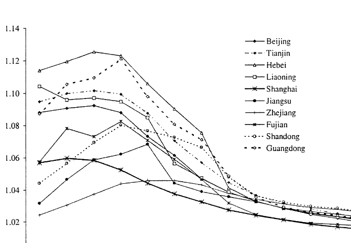
Given these estimates, the performance indicators can then be derived and are reported in Fig. 2. According to this chart, the indicators of FDI performance have moved following an inverted-J shape. It seems that all regions have gone through a learning process lasting for about 3–5 years. In the early 1980s, the regions could on average reduce about 7% of their FDI input. For some regions, the saving could be as high as 13%. However, in the 1990s, FDI performance has become stable and converged across the 10 regions. The improvement in FDI performance has coincided with the massive flow of foreign capital into China since 1992. It is also interesting, but not unexpected, to note that Shanghai has been the best performer since the late 1980s.
4. Summary remarks
In the light of the new growth framework, this paper has investigated the performance of China’s FDI as a factor input. It is found that FDI performance has gone through an inverted J-shape learning process in the past fifteen years. By 1995, all regions have shown relatively efficient use of foreign capital, i.e. less than 3% of overutilisation of FDI. This trend of convergence might be determined by some common factors such as the development of infrastructure, growth of the non-state sector and economic reform. According to official statistical records, over the past decade all regions considered have shown consistent changes in per capita income, the role of the non-state sector and infrastructure
10
development (roads and telephones). Per capita FDI among the regions has also recorded the similar growth pattern. A detailed investigation of the effect of these factors is beyond the scope of the present paper and will be carried out by the author in the near future. In addition, the assumption of ‘radial shrinkage’ of observed inputs in the technique employed could be removed should the price information on all factor inputs be available and reliable. This limitation indicates the scope for more rigorous exercises.
Acknowledgements
Work on this paper was supported by a small grant from the Australian Research Council. The paper also benefited from the helpful comments by an anonymous referee and by seminar participants at the Chunghua Institution for Economic Research, Taipei, June, 1997, and China International Business Symposium, Shanghai, May, 1998.
References
Balasubramanyan, V.N., Salisu, M., Sapsford, D., 1996. Foreign direct investment and growth in EP and IS countries. Economic Journal 106, 92–105.
Coelli, T.J., 1992. A computer program for frontier production function estimation: FRONTIER, Version 2.0. Economics Letters 39, 29–32.
Coelli, T., Perelman, S., 1996. Efficiency measurement, multiple-output technologies and distance functions: With application to European railways, Working Paper No. CREPP 96 / 05, Universite de Liege.
¨
Fare, R., Grosskopf, S., 1990. A distance function approach to price efficiency. Journal of Public Economics 43, 123–126. ¨
Fare, R., Grosskopf, S., 1996. Intertemporal Production Frontiers: With Dynamic DEA, Kluwer Academic Publishers, Boston.
¨
Fare, R., Primont, D., 1995. Multi-output Production and Duality: Theory and Applications, Kluwer Academic Publishers, Boston.
Farrell, M.J., 1957. The measurement of productive efficiency. Journal of the Royal Statistical Society, Series A, General 120, 253–282.
Fried, H., Lovell, C.A.K., Schmidt, S. (Eds.), 1993. The Measurement of Productive Efficiency, Oxford University Press.
10
Grosskopf, S., Hayes, K., 1993. Local public sector bureaucrats and their input choices. Journal of Urban Economics 33, 151–166.
Karikari, J.A., 1992. Causality between direct foreign investment and economic output in Ghana. Journal of Economic Development 17, 7–17.
Krueger, A.O., 1987. Debt, capital flows and LDC Growth. American Economic Review 13, 159–164.
Lovell, C.A. Knox, Richardson, S., Travers, P., Wood, L., 1991. Resources and functions: A new view of inequality in Australia. In: Eichhorn, W. (Ed.), Models and Measurement of Welfare and Inequality, Springer-Verlag, Berlin. Shan, J., Tian, G., Sun, F., 1999. Causality between FDI and economic growth. In: Yanrui, Wu (Ed.), Foreign Direct