ANALYSIS
Aggregation and the role of energy in the economy
Cutler J. Cleveland
a,*, Robert K. Kaufmann
a, David I. Stern
b,1 aCenter for Energy and En6ironmental Studies and Department of Geography,Boston Uni6ersity,675Commonwealth A6enue,Boston,MA02215,USA
bCentre for Resource and En6ironmental Studies,Australian National Uni6ersity,Canberra ACT0200,Australia Received 30 July 1998; received in revised form 30 July 1999; accepted 30 July 1999
Abstract
Methods for investigating the role of energy in the economy involve aggregating different energy flows. A variety of methods have been proposed, but none has received universal acceptance. This paper shows that the method of aggregation has crucial effects on the results of the analysis. We review the principal assumptions and methods for aggregating energy flows: the basic heat equivalents approach, economic approaches using prices or marginal product for aggregation, emergy analysis, and thermodynamic approaches such as exergy. We argue that economic ap-proaches such as the index or marginal product method are superior because they account for differences in quality among fuels. We apply various economic approaches in three case studies in the US economy. In the first, we account for energy quality to assess changes in the energy surplus delivered by the extraction of fossil fuels from 1954 to 1992. The second and third case studies examine the importance of energy quality in evaluating the relation between energy use and GDP. First, a quality-adjusted index of energy consumption is used in an econometric analysis of the causal relation between energy use and GDP from 1947 to 1996. Second, we account for energy quality in an econometric analysis of the factors that determine changes in the energy/GDP ratio from 1947 to 1996. Without adjusting for energy quality, the results imply that the energy surplus from petroleum extraction is increasing, that changes in GDP drive changes in energy use, and that GDP has been decoupled from between aggregate energy use. All of these conclusions are reversed when we account for changes in energy quality. © 2000 Elsevier Science B.V. All rights reserved.
Keywords:Energy aggregation; Energy quality; Economy
www.elsevier.com/locate/ecolecon
1. Introduction
Investigating the role of energy in the economy involves aggregating different energy flows. A va-riety of methods have been proposed, but none is accepted universally. This paper shows that the method of aggregation affects analytical results. We review the principal assumptions and methods
* Corresponding author. Tel.: +1-617-3533083; fax: + 1-617-3535986.
E-mail addresses: [email protected] (C.J. Cleveland), [email protected] (R.K. Kaufmann), [email protected] (D.I. Stern)
1Tel.: +612-62490664; fax: +612-62490757.
for aggregating energy flows: the basic heat equiv-alents approach, economic approaches using prices or marginal product for aggregation, emergy analysis and thermodynamic approaches such as exergy analysis. We argue that economic approaches such as the index or marginal product method are superior because they account for differences in quality among different fuels. We apply economic approaches to three case studies of the US economy. In the first, we account for energy quality to assess changes in the energy surplus delivered by the extraction of fossil fuels from 1954 to 1992. The second and third examine the effect of energy quality on statistical analyses of the relation between energy use and GDP. First, a quality-adjusted index of energy consump-tion is used in an econometric analysis of the causal relation between energy use and GDP from 1947 to 1996. Second, we account for energy quality in an econometric analysis of the factors
that determine changes in the energy/GDP ratio
from 1947 to 1996. Without adjusting for energy quality, the results imply that the energy surplus from petroleum extraction is increasing, that changes in GDP drive changes in energy use, and that GDP has been decoupled from aggregate energy. These conclusions are reversed when we account for changes in energy quality.
2. Energy aggregation and energy quality
Aggregation of primary level economic data has received substantial attention from economists for a number of reasons. Aggregating the vast num-ber of inputs and outputs in the economy makes it easier for analysts to see patterns in the data. Some aggregate quantities are of theoretical inter-est in macro-economics. Measurement of
produc-tivity, for example, requires a method to
aggregate goods produced and factors of produc-tion that have diverse and distinct qualities. For example, the post-War shift towards a more edu-cated work force and from nonresidential struc-tures to producers’ durable equipment required adjustments to methods used to measure labor hours and capital inputs (Jorgensen and Griliches, 1967). Econometric and other forms of
quantita-tive analysis may restrict the number of variables that can be considered in a specific application, again requiring aggregation. Many indexes are possible, so economists have focused on the im-plicit assumptions made by the choice of an index in regard to returns to scale, substitutability, and other factors. These general considerations also apply to energy.
The simplest form of aggregation, assuming that each variable is in the same units, is to add up the individual variables according to their thermal equivalents (BTUs, joules etc.). Eq. (1) illustrates this approach:
Et= % N
i=1
Eit (1)
where Erepresents the thermal equivalent of fuel
i(Ntypes) at timet. The advantage of the thermal equivalent approach is that it uses a simple and well-defined accounting system based on the con-servation of energy, and the fact that thermal equivalents are easily and uncontroversially mea-sured. This approach underlies most methods of energy aggregation in economics and ecology, such as trophic dynamics (Odum, 1957), national energy accounting (US Department of Energy,
1997), energy input – output modeling in
economies (Bullard et al., 1978) and ecosystems
(Hannon, 1973), most analyses of the energy/
GDP relationship (e.g. Kraft and Kraft, 1978) and energy efficiency, and most net energy analy-ses (Chambers et al., 1979).
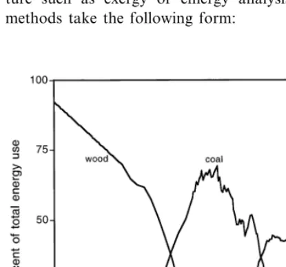
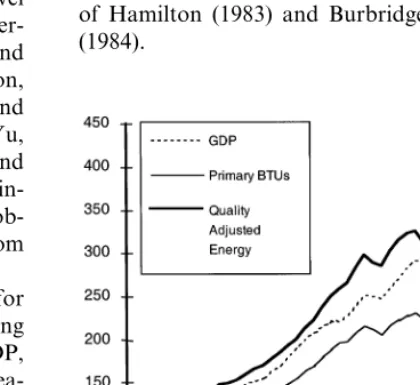
Despite its widespread use, aggregating differ-ent energy types by their heat units embodies a serious flaw: it ignores qualitative differences among energy vectors. We define energy quality as the relative economic usefulness per heat equiv-alent unit of different fuels and electricity. Schurr and Netschert (1960) were among the first to recognize the economic importance of energy quality. Noting that the composition of energy use changes significantly over time (Fig. 1), Schurr and Netschert argued that the general shift to higher quality fuels affects how much energy is required to produce GNP.
energy required to produce a unit of GDP (Schurr and Netschert, 1960; Devine, 1986; Jorgensen, 1986; Rosenberg, 1998). Less attention has been paid to the quality of other fuels, and few studies use a quality-weighting scheme in empirical analy-sis of energy use.
The concept of energy quality needs to be dis-tinguished from that of resource quality (Hall et al., 1986). Petroleum and coal deposits may be identified as high quality energy sources because they provide a very high energy surplus relative to the amount of energy required to extract the fuel. On the other hand, some forms of solar electricity may be characterized as a low quality source because they have a lower energy return on in-vestment (EROI). However, the latter energy vec-tor may have higher energy quality because it can be used to generate more useful economic work than one heat unit of petroleum or coal.
Taking energy quality into account in energy aggregation requires more advanced forms of ag-gregation. Some of these forms are based on concepts developed in the energy analysis litera-ture such as exergy or emergy analysis. These methods take the following form:
E*t= % N
i=1
litEit (2)
where the l’s are quality factors that may vary
among fuels and over time for individual fuels. In the most general case that we consider, an aggre-gate index can be represented as:
f(Et)=%
N
i=1
litg(Eit) (3)
where f() and g() are functions, lit are weights, theEiare theNdifferent energy vectors andEtis
the aggregate energy index in period t. An
exam-ple of this type of indexing is the Discrete Divisia Index or Tornquist-Theil Index described below.
3. Economic approaches to energy quality
From an economic perspective, the value of a heat equivalent of fuel is determined by its price. Price-taking consumers and producers set mar-ginal utilities and products of the different energy vectors equal to their market prices. These prices and their marginal productivities and utilities are set simultaneously in general equilibrium. The value marginal product of a fuel in production is the marginal increase in the quantity of a good or service produced by the use of one additional heat unit of fuel multiplied by the price of that good or service. We can also think of the value of the
marginal product of a fuel in household
production.
The marginal product of a fuel is determined in
partby a complex set of attributes unique to each
fuel such as physical scarcity, capacity to do useful work, energy density, cleanliness, amenabil-ity to storage, safety, flexibilamenabil-ity of use, cost of conversion, and so on. But the marginal product is not uniquely fixed by these attributes. Rather, the energy vector’s marginal product varies ac-cording to the activities in which it is used, how much and what form of capital, labor, and mate-rials it is used in conjunction with, and how much energy is used in each application. As the price rises due to changes on the supply-side, users can reduce their use of that form of energy in each activity, increase the amount and sophistication of capital or labor used in conjunction with the fuel,
or stop using that form of energy for lower value activities. All these actions raise the marginal productivity of the fuel. When capital stocks have to be adjusted, this response may be somewhat sluggish and lead to lags between price changes and changes in the value marginal product.
The heat equivalent of a fuel is just one of the attributes of the fuel and ignores the context in which the fuel is used, and thus cannot explain, for example, why a thermal equivalent of oil is more useful in many tasks than is a heat equiva-lent of coal (Adams and Miovic, 1968; Mitchell, 1974; Webb and Pearce, 1975). In addition to attributes of the fuel, marginal product also de-pends on the state of technology, the level of other inputs, and other factors. According to neoclassical theory, the price per heat equivalent of fuel should equal its value marginal product, and, therefore, represent its economic usefulness. In theory, the market price of a fuel reflects the myriad factors that determine the economic use-fulness of a fuel from the perspective of the end-user.
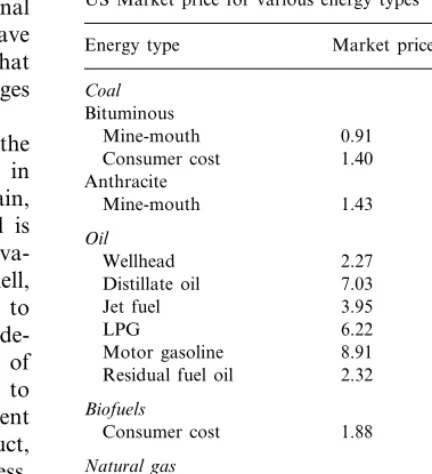
Consistent with this perspective, the price per heat equivalent of fuel varies substantially among fuel types (Table 1). The different prices demon-strate that end-users are concerned with attributes other than heat content. As Berndt (1978) states:
Because of [the] variation in attributes among energy types, the various fuels and electricity are less than perfectly substitutable — either in production or consumption. For example, from the point of view of the end-user, a Btu of coal is not perfectly substitutable with a Btu of electricity; since the electricity is cleaner, lighter, and of higher quality, most end-users are will-ing to pay a premium price per Btu of
electric-ity. However, coal and electricity are
substitutable to a limited extent, since if the premium price for electricity were too high, a substantial number of industrial users might switch to coal. Alternatively, if only heat con-tent mattered and if all energy types were then perfectly substitutable, the market would tend to price all energy types at the same price per Btu (p. 242).
Table 1
US Market price for various energy typesa
Energy type Market price ($/106btu) Coal Residual fuel oil 2.32 Biofuels
aSource: Department of Energy (1997). Values are 1994 prices.
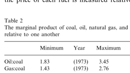
relative marginal product and relative price, and that several years of adjustment are needed to bring this relation into equilibrium. The results are summarized in Table 2, and suggest that over time prices do reflect the marginal product — and hence the economic usefulness — of fuels.
Other analysts calculate the average product of fuels, which is a close proxy for marginal prod-ucts. Adams and Miovic (1968) estimate a pooled annual cross-sectional regression model of indus-trial output as a function of fuel use in seven European economies from 1950 to 1962. Their results indicate that petroleum is 1.6 – 2.7 times more productive than coal in producing industrial output. Electricity is 2.7 – 14.3 times more produc-tive than coal. Using a regression model of the
energy/GDP ratio in the US, Cleveland et al.
(1984) find that the quality factors of petroleum and electricity relative to coal were 1.9 and 18.3, respectively.
3.1. Price-based aggregation
If marginal product is related to its price, en-ergy quality can be measured by using the price of fuels to weight their heat equivalents. The sim-plest approach defines the weighting factor (l’s) in Eq. (2) as:
lit=
Pit
P1t
(4)
wherePitis the price per Btu of fuel. In this case, the price of each fuel is measured relative to the
price of fuel type 1. Turvey and Nobay (1965) use Eq. (3) to aggregate fuel use in the UK.
The quality index in Eq. (4) embodies a restric-tive assumption — that fuels are perfect substi-tutes — and the index is sensitive to the choice of numeraire (Berndt, 1978; Stern, 1993). Because fuels are not perfect substitutes, a rise in the price of one fuel relative to the price of output will not be matched by equal changes in the prices of the other fuels relative to the price of output. For example, the rise in oil prices in 1979 – 80 would cause an aggregate energy index which uses oil as the numeraire to fall dramatically. An index that uses coal as the numeraire would show a large fall in 1968 – 74, one not indicated by the oil-based index.
To avoid dependence on a numeraire, Berndt (1978, 1990) proposed a discrete approximation to the Divisia index to aggregate energy. The for-mula for constructing the discrete Divisia index
E* is:
quantity of BTU for each fuel in final energy use. Note that prices enter the Divisia index via cost or expenditure shares. The Divisia index permits variable substitution among material types with-out imposing a priori restrictions on the degree of
substitution (Diewert, 1976). Diewert (1976)
shows that this index is an exact index number representation of the linear homogeneous translog production function where fuels are homotheti-cally weakly separable as a group from the other factors of production. With reference to equation (3) f()=g()=Dln(), whilelitis given by the aver-age cost share over the two periods of the differ-encing operation.
Table 2
The marginal product of coal, oil, natural gas, and electricity relative to one another
Minimum Year Maximum Year 1.83
Oil:coal (1973) 3.45 (1990)
1.43
Gas:coal (1973) 2.76 (1944)
(1944)
0.97 (1933) 1.45 (1992) Oil:gas
(1930) Electric- 1.75 (1991) 6.37
ity:oil
2.32 (1986) 6.32 (1930)
3.2. Discussion
Aggregation using price has its shortcomings. Lau (1982) suggests that prices provide a reason-able method of aggregation if the aggregate cost function is homothetically separable in the raw material input prices. This means that the elastic-ity of substitution between different fuels is not a function of the quantities of non-fuel inputs used. This may be an unrealistic assumption in some cases. Also, the Divisia index assumes that the substitution possibilities among all fuel types and output are equal.
Another limit on the use of prices is that they generally do not exist for wastes. Thus, an eco-nomic index of waste flows is impossible to construct.
It is well-known that energy prices do not reflect their full social cost due to a number of market imperfections. This is particularly true for the environmental impact caused by their extrac-tion and use. These problems lead some to doubt the usefulness of price as the basis for any indica-tor of sustainability (Hall, 1990; Odum, 1996). But with or without externalities, prices should reflect productivities. Internalizing externalities will shift energy use, which, in turn, will then change marginal products.
Moreover, prices produce a ranking of fuels (Table 1) that is consistent with our intuition and with previous empirical research (Schurr and Netschert, 1960; Adams and Miovic, 1968; Cleve-land et al., 1984; Kaufmann, 1991). One can conclude that government policy, regulations, cartels and externalities explain some of the price differentials among fuels, but certainly not the substantial ranges that exist. More fundamentally, price differentials are explained by differences in attributes such as physical scarcity, capacity to do useful work, energy density, cleanliness, amenabil-ity to storage, safety, flexibilamenabil-ity of use, cost of conversion, and so on. Wipe away the market imperfections and the price per BTU of different energies would vary due to the different combina-tions of attributes that determine their economic usefulness. The different prices per BTU indicate that users are interested in attributes other than heat content.
4. Alternative approaches to energy aggregation
While we argue that the more advanced eco-nomic indexing methods, such as Divisia aggrega-tion, are the most appropriate way to aggregate energy use for investigating its role in the econ-omy, the ecological economics literature proposes other methods of aggregation. We briefly review two of these methods in this section and assess limits on their ability to aggregate energy use.
5. Exergy
Ayres et al. (1996) and Ayres and Martin˜as (1995) propose a system of aggregating energy and materials based on exergy. Exergy measures the useful work obtainable from an energy source or material, and is based on the chemical energy embodied in the material or energy, based on its physical organization relative to a reference state. Thus, exergy measures the degree to which a material is organized relative to a random assem-blage of material found at an average concentra-tion in the crust, ocean or atmosphere. The higher the degree of concentration, the higher the exergy content. The physical units for exergy are the same as for energy or heat, namely kilocalories, joules, BTUs, etc. For fossil fuels, exergy is nearly equivalent to the standard heat of combustion; for other materials specific calculations are needed that depend on the details of the assumed conver-sion process.
ani-mals or inanimate source is converted into final services. A low exergy efficiency implies potential for efficiency gains for converting energy and materials into goods and services. Similarly, the ratio of exergy embodied in material wastes to exergy embodied in resource inputs is the ‘most general measure of pollution’ (Ayres et al., 1996). Ayres and Martin˜as (1995) also argue that the exergy of waste streams is a proxy for their poten-tial ecotoxicity or harm to the environment, at least in general terms.
From an accounting perspective, exergy is ap-pealing because it is based on the science and laws of thermodynamics and thus has a well-estab-lished system of concepts, rules, and information that are available widely. But like enthalpy, ex-ergy should not be used to aggregate enex-ergy and material inputs to construct economic indicators because it is one-dimensional. Like enthalpy, ex-ergy does not vary with, and hence does not necessarily reflect attributes of fuels that deter-mine their economic usefulness, such as energy density, cleanliness, cost of conversion, and so on. The same is true for materials. Exergy cannot explain, for example, impact resistance, heat
resis-tance, corrosion resistance, stiffness, space
maintenance, conductivity, strength, ductility, or other properties of metals that determine their usefulness. Like prices, exergy does not reflect all the environmental costs of fuel use. The exergy of coal, for example, does not reflect coal’s contribu-tion to global warming or its impact on human health relative to, say, natural gas. As Ayres (1995) and Martin˜as note, the exergy of wastes is at best a rough first-order approximation of envi-ronmental impact because it does not vary with the specific attributes of a waste material and its receiving environment that cause harm to organ-isms or that disrupt biogeochemical cycles. In theory exergy can be calculated for any energy or material, but in practice, the task of assessing the hundreds (thousands?) of primary and intermedi-ate energy and mintermedi-aterial flows in an economy is daunting.
5.1. Emergy
Odum (1996) analyzes energy and materials
with a system that traces their flows within and between society and the environment. It is impor-tant to differentiate between two aspects of Odum’s contribution. The first is his development of a biophysically-based, systems-oriented model of the relationship between society and the envi-ronment. Here Odum’s (1971; Odum and Odum, 1976) early contributions helped lay the founda-tion for the biophysical analysis of energy and material flows, an area of research that forms part of the intellectual backbone of ecological econom-ics (Martinez-Alier, 1987; Krishnan et al., 1995; Costanza et al., 1997). The insight from this part of Odum’s work is illustrated by the fact that ideas he emphasized — energy and material flows, feedbacks, hierarchies, thresholds, time lags — are key concepts of the analysis of sustainabil-ity in a variety of disciplines.
The second aspect of Odum’s work, which we are concerned with here, is a specific empirical issue: the identification, measurement, and aggre-gation of energy and material inputs to the econ-omy, and their use in the construction of indicators of sustainability. Odum measures, val-ues, and aggregates energy of different types by their transformities. Transformities are calculated as the amount of one type of energy required to produce a heat equivalent of another type of energy. To account for the difference in quality of thermal equivalents among different energies, all energy costs are measured in solar emjoules (sej), the quantity of solar energy used to produce another type of energy. Fuels and materials with higher transformities require larger amounts of sunlight to produce and therefore are considered more economically useful (Odum, 1996).
that determine its usefulness relative to other fuels. It is hard to imagine how this set of attributes is in general related to — much less determined by — the amount of solar energy required to produce coal. Second, the emergy methodology is inconsis-tent with its own basic tenant, namely that quality varies with embodied energy or emergy. Coal deposits that we currently extract were laid down over many geological periods that span half a billion years (Tissot, 1979). Coals thus have vastly different embodied emergy, but only a single trans-formity for coal is normally used. Third, the emergy methodology depends on plausible but arbitrary choice of conversion technologies (e.g. boiler effi-ciencies) that assume users choose one fuel relative to another and other fuels based principally on their relative conversion efficiencies in a particular application. Finally, the emergy methodology relies on long series of calculations with data that vary in quality. Yet little attention is paid to the sensi-tivity of the results to data quality and uncertainty, leaving the reader with little no sense of how precise or reliable the emergy calculations are.
6. Case study 1: net energy from fossil fuel extraction in the US
One technique for evaluating the productivity of energy systems is net energy analysis, which com-pares the quantity of energy delivered to society by an energy system to the energy used directly and indirectly in the delivery process. Cottrell (1955), Odum (1971) and Odum and Odum (1976) were the first to identify the economic importance of net energy. Energy return on investment (EROI) is the ratio of energy delivered to energy costs (Cleveland et al., 1984). There is a long debate about the relative strengths and weaknesses of net energy analysis.2
One restriction on net energy analysis’ ability to deliver the insights it promises is its
treatment of energy quality. In most net energy analyses, inputs and outputs of different types of energy are aggregated by their thermal equivalents. Following (Cleveland, 1992), this case study illus-trates how accounting for energy quality affects calculations for the EROI of the US petroleum sector from 1954 to 1992.
6.1. Methods and data
Following the definitions in Eq. (2), a quality-corrected EROI is defined by:
EROIt*=
t and Eo and Ec are the thermal equivalents of
energy outputs and energy inputs, respectively. We construct Divisia indices for energy inputs and outputs to account for energy quality in the numer-ator and denominnumer-ator. The prices for energy out-puts (oil, natural gas, natural gas liquids) and energy inputs (natural gas, gasoline, distillate fuels, coal, electricity) are the prices paid by industrial end-users for each energy type (US Department of Energy, 1997).
Cleveland (1992) provides full details on the data and methods presented here. Energy inputs include only industrial energies: the fossil fuel and electric-ity used directly and indirectly to extract petroleum. The costs include only those energies used to locate and extract oil and natural gas and prepare them for shipment from the wellhead. Transportation and refining costs are excluded from this analysis. Output in the petroleum industry is the sum of the marketed production of crude oil, natural gas, and natural gas liquids.
The direct energy cost of petroleum is the fuel and electricity used in oil and gas fields (Bureau of Census, various years). Indirect energy costs include the energy used to produce material in-puts and to produce and maintain the capital used to extract petroleum. The indirect energy cost of materials and capital is calculated from data for the dollar cost of those inputs to petroleum extraction processes. Energy cost of capital and
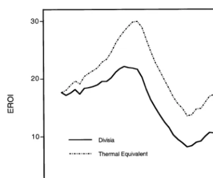
Fig. 2. Energy return on investment (EROI) for petroleum extraction in the US, with energy inputs and outputs measured in heat equivalents and a Divisia index.
Thus, the two highest quality fuels, electricity and refined oil products, comprise a large and growing fraction of the denominator in the Divisia EROI compared to the thermal equivalent EROI. Thus the Divisia denominator increases faster than the heat-equivalent denominator, causing EROI to decline faster in the former case.
7. Case study 2: causality in the energy – GDP relationship
One of the most important questions about the environment – economy relationship is the strength of the linkage between economic growth and en-ergy use. With a few exceptions (Cleveland et al., 1984; Berndt, 1990; Kaufmann, 1991; Stern, 1993; Patterson, 1996), most analyses ignore the effect of energy quality in the assessment of this rela-tionship. One statistical approach to address this question is Granger causality and/or cointegration analysis (Granger, 1969; Engle and Granger,
1987).3 Granger causality tests whether (1) one
variable in a relation can be meaningfully de-scribed as a dependent variable and the other variable an independent variable; (2) the relation is bi-directional; or (3) no meaningful relation exists at all. This is usually done by testing whether lagged values of one of the variables adds significant explanatory power to a model which already includes lagged values of the dependent variable and perhaps also lagged values of other variables.
While Granger causality can be applied to both stationary and integrated time series (time series which follow a random walk), cointegration ap-plies only to linear models of integrated time series. The irregular trend in integrated series is known as a stochastic trend as opposed to a simple linear deterministic time trend. Time series of GDP and energy use usually are found to be integrated. Cointegration analysis aims to uncover causal relations among variables by determining if the stochastic trends in a group of variables are shared by the series so that the total number of materials is defined as the dollar cost of capital
depreciation and materials times the energy inten-sity of capital and materials (BTU/$). The energy intensity of capital and materials is measured by the quantity of energy used to produce a dollar’s worth of output in the industrial sector of the US economy. That quantity is the ratio of fossil fuel and electricity use to real GDP produced by industry (US Department of Energy, 1997).
6.2. Results and conclusions
The thermal equivalent and Divisia EROI for petroleum extraction show significant differences (Fig. 2). The quality-corrected EROI declines faster than the thermal-equivalent EROI. The thermal-equivalent EROI increases by 60% rela-tive to the Divisia EROI between 1954 and 1992. This difference is driven largely by changes in the mix of fuel qualities in energy inputs. Electricity, the highest quality fuel, is an energy inputs but not an energy output. Its share of total energy use rises from 2 to 12% over the period; its cost share increases from 20 to 30%. Thus, in absolute terms the denominator in the Divisia EROI is weighted more heavily than in the thermal equivalent EROI. The Divisia-weighted quantity of refined oil products is larger than that for gas and coal.
unique trends is less than the number of vari-ables. It can also be used to test if there are residual stochastic trends which are not shared by any other variables. This may be an indica-tion that important variables have been omitted from the regression model or that the variable with the residual trend does not have long-run interactions with the other variables.
Either of these conclusions could be true should there be no cointegration. The presence of cointegration can also be interpreted as the presence of a long-run equilibrium relationship between the variables in question. The parame-ters of an estimated cointegrating relation are called the cointegrating vector. In multivariate models there may be more than one such cointegrating vector.
7.1. Granger causality and the energy GDP relation
A series of analysts use statistical tests devel-oped by Granger (1969) or Sims (1972) to
eval-uate whether energy use or energy prices
determine economic growth, or whether the level of output in the US and other economics deter-mine energy use or energy prices (Kraft and Kraft, 1978; Akarca and Long, 1980; Hamilton, 1983; Burbridge and Harrison, 1984; Yu and Hwang, 1984; Yu and Choi, 1985; Erol and Yu,
1987; Ammah-Tagoe, 1990; Abosedra and
Baghestani, 1991). Generally, the results are in-conclusive. Where significant results are ob-tained, they indicate causality running from output to energy use.
Stern (1993) tests US data (1947 – 1990) for Granger causality in a multivariate setting using a vector autoregression (VAR) model of GDP, energy use, capital, and labor inputs. He mea-sures energy use by its thermal equivalents and the Divisia aggregation method discussed above. The relation among GDP, the thermal equiva-lent of energy use, and the Divisia energy use indicates that there is less ‘decoupling’ between GDP and energy use when the aggregate mea-sure for energy use accounts for qualitative dif-ferences (Fig. 3). The multivariate methodology is important because changes in energy use
fre-quently are countered by substitution with labor and/or capital and thereby mitigate the effect of changes in energy use on output. Weighting en-ergy use for changes in the composition of the energy input is important because a large part of the growth effects of energy are due to sub-stitution of higher quality energy sources such as electricity for lower quality energy sources such as coal (Jorgenson, 1984; Hall et al., 1986) (Fig. 1).
Bivariate tests of Granger causality show no causal order in the relation between energy and GDP in either direction regardless of the mea-sure used to qualify energy use (Table 3). In the multivariate model with energy measured in pri-mary BTUs, GDP was found to ‘Granger cause’ energy use. However, when both innovations — a multivariate model and energy use is adjusted for quality — are employed, energy ‘Granger causes’ GDP. These results show that adjusting energy for quality is important as is considering the context within which energy use is occur-ring. The result that energy use plays an impor-tant role in determining the level of economic activity is consistent with the price-based studies of Hamilton (1983) and Burbridge and Harrison (1984).
Table 3
Energy GDP causality tests USA 1947–1990a
Multivariate model Bivariate model
Quality adjusted energy
Primary BTUs Primary BTUs Quality adjusted energy
0.9657 0.5850
Energy causes 0.8328 3.1902
0.4402 0.5628
0.4428 0.3188E-01
GDP
0.3421
GDP Causes 0.7154 9.0908 0.8458
0.5878
Energy 0.7125 0.7163E-03 0.5106
aThe test statistic is an F statistic. Significance levels in italics. A significant statistic indicates that there is Granger causality in the direction indicated.
7.2. Cointegration and the energy GDP relation
Stern (1998) tests for cointegration between en-ergy use and economic activity in the same multi-variate model used in Stern (1993) with US data from 1948 to 1994. If a multivariate approach helps uncover the direction of Granger causality between energy and GDP, then a multivariate approach should clarify the cointegrating rela-tions among variables. The Johansen methodol-ogy (Johansen, 1988; Johansen and Juselius, 1990) is used to test for the number of cointegrating vectors in the multivariate Vector Error Correc-tion Model (VECM) estimate their parameters, and the rate at which energy use and economic activity adjusts to disequilibrium in the long-run relations. The VECM is given by:
Dyt=g+ab%[1,t,yt−1]%+GiDyt−i+ot (7) in whichyis a vector of variables (in logarithms),
otis a vector of random disturbances,Dis the first difference operator,tis a deterministic time trend,
gis a vector of coefficients to be estimated,ais a matrix of adjustment coefficients (to be
esti-mated), b is the matrix of cointegrating vectors
(to be estimated), and the Gi are matrices of
short-run dynamics coefficients (to be estimated). The test for the number of cointegrating vectors
determines the dimensions of aand b.
The cointegrating vectors indicate that energy use and GDP are present in both cointegrating relations but the elements ofaindicate that these cointegrating relations affect the equation for en-ergy use only. This result indicates that there is a statistically significant relation between energy use
and GDP, but the direction of causality runs from economic activity to energy use. This result is consistent with Stern (1993).
Table 4 presents the results for the model using the quality-adjusted energy index. The third row in Table 4 presents tests for excluding each of the variables from the long-run relation. Restrictions that eliminate energy from the long-run relation-ships are rejected while the same restrictions for capitol cannot be rejected. However, the statistics in the fourth row show that none of the variables can be treated as exogenous variables. The causal pattern is in general mutual. The fifth and sixth rows show the signs and significance of the adjust-ment coefficients. The first cointegrating relation has no significant effect on the capital equation. However, all the other coefficients are significant. This again confirms the mutual causality pattern. Use of quality adjusted energy indices clearly has an important effect on analyses of Granger causality and cointegration. When energy is mea-sured in thermal equivalents, research predomi-nantly finds that either there is no relation between energy and GDP or that the relation runs from GDP to energy in both bivariate and multi-variate models. The implications for the impor-tance of energy in the economy are quite different in the two cases.
8. Case study 3: the determinants of the energy – GDP relationship
energy use to total economic activity, or the energy/
real GDP ratio (E/GDP ratio). This ratio has
declined since 1950 in many industrial nations. Controversy arises regarding the interpretation of this decline. Many economists and energy analysts argue that the declines indicate that the relation between energy use and economic activity is rela-tively weak. This interpretation is disputed by many biophysical economists. They argue that the decline in theE/GDP ratio overstates the ability to decouple energy use and economic activity because many
analyses of the E/GDP ratio ignore the effect of
changes in energy quality (Fig. 1).
The effect of changes in energy quality (and changes in energy prices, and types of goods and
services produced and consumed) on the E/GDP
ratio can be estimated using Eq. (6), which was developed by Gever et al. (1986) and Cleveland et al. (1984):
in whichEis the total primary energy consumption
(measured in heat units), GDP is real GDP, Primary electricity is electricity generated from hydro,
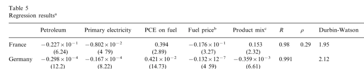
nu-clear, solar, or geothermal sources, PCE is real personal consumption expenditures spent directly on energy by households, Product mix measures the fraction of GDP that originates in energy intensive sectors (e.g. chemicals) or nonenergy intensive sectors (e.g. services), and Price is a measure of real energy prices. Kaufmann (1992) applied this model to France, Germany, Japan and the United King-dom.
The effect of energy quality on theE/GDP ratio
is measured by the fraction of total energy consump-tion from individual fuels. The sign on the regression coefficientsb1,b2, andb3is expected to be negative
because natural gas, oil, and primary electricity can do more useful work (and therefore generate more economic output) per heat unit than coal. The rate at which an increase in the use of natural gas, oil, or primary electricity reduces theE/GDP ratio is not constant. Engineering studies indicate that the efficiency with which energies of different types are converted to useful work depends on their use. Petroleum can provide more motive power per heat unit of coal, but this advantage nearly disappears if petroleum is used as a source of heat (Adams and Miovic, 1968). From an economic perspective, the law of diminishing returns implies that the first uses of high quality energies are directed at tasks that are best able to make use of the physical, technical, and economic aspects of an energy type that combine to determine its high quality status. As the use of a high quality energy source expands, it
Table 4
Cointegration modela
ln GDP ln Energy
Variables ln Capital ln Labor Trend
−1.174 0.354
Coefficients of the first cointegrating vector −0.191 1 0.014
−0.689 −0.009 −0.157
−0.237 1
Coefficients of the second cointegrating vector
13.24 11.48
Chi-square test statistic for exclusion of variable from the 18.08 1.62 17.92 cointegration space (5% critical level=5.99)
11.80 16.13 8.18 16.27 –
Chi-square test statistic for weak exogeneity of the variables (5% critical level=5.99)
0.046 0.053
First column of alpha (tstats in parentheses) −0.005 0.087 (4.239) – (2.005) (2.150) (−0.974)
1.624 0.229 0.801 –
1.155 Second column of alpha (tstats in parentheses)
is used for tasks that are less able to make use of the attributes that confer high quality. The combi-nation of physical differences in the use of energy and the economic ordering in which they are applied to these tasks implies that the amount of economic activity generated per heat unit dimin-ishes as the use of a high quality energy expands. Diminishing returns on energy quality is imposed on the model by specifying the fraction of the energy budget from petroleum, primary electric-ity, natural gas, or oil in natural logarithms. This specification ensures that the first uses of high
quality energies decreases the energy/GDP ratio
faster than the last uses.
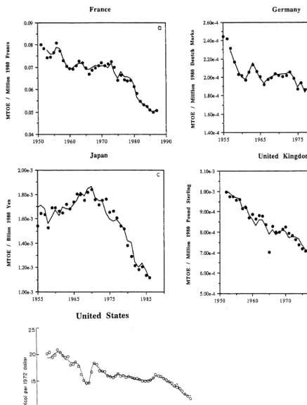
The regression results (Table 5) indicate that Eq. (6) can be used to account for most of the
variation in the energy/GDP ratio for France,
Germany, Japan, and the UK during the post-war period (Kaufmann, 1992) and in the US since 1929 (Cleveland et al., 1984; Gever et al., 1986; Kaufmann, 1994). All of the variables have the sign as expected by economic theory, are statisti-cally significant, and the error terms have the properties assumed by the estimation technique.
Analysis of regression results indicate that changes in energy mix can account for a
signifi-cant portion of the downward trend in E/GDP
ratios. The change from coal to petroleum and petroleum to primary electricity is associated with
a general decline in the E/GDP ratio in France,
Germany, the UK, and the US during the post-war period (Fig. 4a – d). The fraction of total energy consumption that is supplied by petroleum increases steadily in each nation through the early 1970s. After the first oil shock, the fraction of total energy use from petroleum is steady or declines slightly in these four nations. However,
energy mix continues to reduce the energy/real
GDP ratio after the first oil shock because the fraction of total energy use from primary electric-ity rises steadily. The effect of changes in energy
mix on the E/GDP ratio shows no trend over
time in Japan, where the fraction of total energy consumption that is supplied by primary electric-ity falls through the early 1970s and increases steadily thereafter. This U shape offsets the steady increase in the fraction of total energy use from petroleum that occurs prior to 1973 (Table 5).
These regression results indicate that the
histor-ical reduction in the E/GDP ratio is associated
with shifts in the types of energies used and the types of goods and services consumed and pro-duced. Diminishing returns to high quality ener-gies and the continued consumption of goods from energy-intensive sectors such as manufactur-ing imply that the ability for changes in the composition of inputs and outputs to reduce the energy/real GDP ratio further are limited.
9. Conclusions and implications
J
.
Cle
6
eland
et
al
.
/
Ecological
Economics
32
(2000)
301
–
317
315
Table 5
Regression resultsa
Fuel priceb Product mixc R r Durbin-Watson Estimation period Primary electricity
Petroleum PCE on fuel
0.98
France −0.227×10⁻¹ −0.802×10⁻² 0.394 −0.176×10⁻¹ 0.153 0.29 1.95 1953–1987 (2.32)
(6.24) (4 79) (2.89) (3.27)
−0.359×10⁻³
−0.298×10⁻⁴ −0.167×10⁻⁴ 0.421×10⁻² −0.132×12−7 0.991 2.12 1957–1986 Germany
(12.2) (8.22) (14.73) (4 59) (6.61)
0.953 0.47 2.26 1955–1986 0.253×10⁻⁴
.0423×10−1 −.320×10−3 Japan −0.235×10⁻³ −0.302×10⁻³
(3.11)
(2.83) (4.28) (3.30) (5.83)
0.968
UK −0.883×10⁻³ −.705×10−4 0.124×10⁻¹ 0.159×10⁻² 1.82 1952–1986 (9 09)
(3.88) (4.67) (2.54)
at, Statistic in parentheses.
bFuel price, France (0–1); Germany (1–2); Japan (–2). Running average in parentheses.
The manner in which these improvements have been largely achieved should give pause for thought. If decoupling is largely illusory, any rise in the cost of producing high quality energy vectors could have important economic impacts. Such an increase might occur if use of low cost coal to generate electricity is restricted on
envi-ronmental, in particular climate change,
grounds. If the substitution process cannot
con-tinue, further reductions in the E/GDP ratio
would slow. Three factors might limit future substitution to higher quality energy. First, there are limits to the substitution process. Eventually all energy used would be of the highest quality variety — electricity — and no further substitu-tion could occur. Future discovery of a yet higher quality energy source might mitigate this but it would be unwise to rely on the discovery of new physical principles. Second, as different energy sources are not perfect substitutes, the substitution process could have economic limits that will prevent full substitution. For example, it is difficult to imagine an airliner running on electricity. Third, it is likely that supplies of petroleum — which is of higher quality than coal — will begin to decline fairly early in the next century.
Finally, our conclusions do not imply that
one-dimensional and/or physical indicators are
universally inferior to the economic indexing ap-proach we endorse. As one reviewer noted, ecol-ogists might raise the problem of Leibig’s law of the minimum in which the growth or sustain-ability of a system is constrained by that single critical element in least supply. Exergy or mass are appropriate if the object of analysis is a single energy or material flux. Physical units are also necessary to valuate those flows. Integrated assessment of a material cycle within and be-tween the environment and the economy is
logi-cally based on physical stocks and flows.
However, when the question being asked re-quires the aggregation of energy flows in eco-nomic systems, an ecoeco-nomic approach such as Divisa aggregation or a direct measure of mar-ginal product embody a more tenable set of
as-sumptions than does aggregation by
one-dimensional approaches.
References
Abosedra, S., Baghestani, H., 1991. New evidence on the causal relationship between United States energy con-sumption and gross national product. J. Ener. Devel. 14, 285 – 292.
Adams, F.G., Miovic, P., 1968. On relative fuel efficiency and the output elasticity of energy consumption in west-ern Europe. J. Ind. Econ. 17, 41 – 56.
Akarca, A., Long, T., 1980. On the relationship between energy and GNP: a reexamination. J. Ener. Devel. 5, 326 – 331.
Ammah-Tagoe F.A., 1990. On woodfuel, total energy con-sumption and GDP in Ghana: a study of trends and causal relations. Center for Energy and Environmental Studies, Boston University, Boston, MA (mimeo). Ayres, R., Martin˜as, K., 1995. Waste potential entropy: the
ultimate ecotoxic? Econ. Appl. 48, 95 – 120.
Ayres, R.U., Ayres, L.W., Martinas, K., 1996. Eco-thermo-dynamics: exergy and life cycle analysis. INSEAD, Cen-ter for the Management of Environmental Resources. Working Paper 961041.
Berndt, E.R., 1978. Aggregate energy, efficiency and produc-tivity measurement. Annu. Rev. Energy 3, 225 – 273. Berndt, E., 1990. Energy use, technical progress and
produc-tivity growth: a survey of economic issues. J. Prod. Anal. 2, 67 – 83.
Bullard, C.W., Penner, P.S., Pilati, D.A., 1978. Net energy analysis: a handbook for combining process and input – output analysis. Resourc. Ener. 1, 267 – 313.
Burbridge, J., Harrison, A., 1984. Testing for the effects of oil prices rises using vector autoregressions. Int. Econ. Rev. 25, 459 – 484.
Chambers, R.S., Herendeen, R.A., Joyce, J.J., Penner, P.S., 1979. Gasohol: does it or doesn’t it provide positive net energy? Science 206, 789 – 795.
Cleveland, C.J., 1992. Energy quality and energy surplus in the extraction of fossil fuels in the US. Ecol. Econ. 6, 139 – 162.
Cleveland, C.J., Costanza, R., Hall, C.A.S., Kaufmann, R., 1984. Energy and the U.S. economy: a biophysical per-spective. Science 255, 890 – 897.
Costanza, R., Cleveland, C., Perrings, C. (Eds.), 1997. The Development of Ecological Economics. Edwin Elgar, London.
Cottrell, W.F., 1955. Energy and Society. McGraw-Hill, New York, p. 330.
Devine, W.D., 1986. Historical perspective on electrification in manufacturing. In: Schurr, S.H., Sonenblum, S. (Eds.), Electric Power Research Institute, Electricity Use, Pro-ductive Efficiency and Economic growth, pp. 131 – 164. Diewert, W.E., 1976. Exact and superlative index numbers.
J. Econ. 4, 115 – 146.
Erol, U., Yu, E.S.H., 1987. On the causal relationship between energy and income for industrialized countries. J. Ener. Devel. 13, 113 – 122.
Gever, J., Kaufmann, R., Skole, D., Vorosmarty, C., 1986. Beyond Oil: The Threat to Food and Fuel in the Coming Decades. Ballinger, Cambridge, p. 304.
Granger, C.W.J., 1969. Investigating causal relations by econometric models and cross-spectral methods. Econo-metrica 37, 424 – 438.
Hall, C.A.S., Cleveland, C.J., Kaufmann, R.K., 1986. Energy and Resource Quality: The Ecology of the Economic Pro-cess. Wiley Interscience, New York.
Hall, C.A.S., 1990. Sanctioning resource depletion: economic development and neoclassical economics. The Ecol. 20, 99 – 104.
Hamilton, J.D., 1983. Oil and the macroeconomy since World War II. J. Polit. Econ. 91, 228 – 248.
Hannon, B., 1973. The structure of ecosystems. J. Theoret. Biol. 41, 535 – 546.
Johansen, S., Juselius, K., 1990. Maximum likelihood estima-tion and inference on cointegraestima-tion with applicaestima-tion to the demand for money. Ox. Bull. Econ. Stat. 52, 169 – 209. Johansen, S., 1988. Statistical analysis of cointegration vectors.
J. Econ. Dynam. Contr. 12, 231 – 254.
Jorgensen, D.W., Griliches, Z., 1967. The explanation of pro-ductivity change. Rev. Econ. Stud. 34, 249 – 282. Jorgensen, D.W., 1986. The role of energy in productivity
growth. In: Schurr, S.H., Sonenblum, S. (Eds.), Electric Power Research Institute, Electricity Use, Productive Effi-ciency and Economic growth, pp. 43 – 92.
Jorgenson, D.W., 1984. The role of energy in productivity growth. Ener. J. 5 (3), 11 – 26.
Kaufmann, R.K., 1992. A biophysical analysis of the energy/ real GDP ratio: implications for substitution and technical change. Ecol. Econ. 6, 35 – 56.
Kaufmann, R.K., 1994. The relation between marginal product and price in US energy markets. Ener. Econ. 16, 145 – 158.
Kraft, J., Kraft, A., 1978. On the relationship between energy and GNP. J. Ener. Devel. 3, 401 – 403.
Krishnan, R., Harris, J.M., Goodwin, N.R. (Eds.), 1995. A Survey of Ecological Economics. Island Press, Washing-ton, DC, p. 384.
Lau, L.J., 1982. The measurement of raw material inputs. In: Smith, V.K., Krutilla, J.V. (Eds.), Explorations in Natural Resource Economics. The Johns Hopkins University Press, Baltimore, pp. 167 – 200.
Linde, D.R. (Ed.), 1991 – 1992. CRC Handbook of Chemistry
and Physics, 72nd Edition, CRC Press, Boca Raton, Ann Arbor, Boston.
Martinez-Alier, J., 1987. Ecological Economics. Basil Black-well, Oxford, p. 286.
Mitchell, E.J., 1974. US Energy Policy: A Primer. American Enterprise Institute for Public Policy Research, Washing-ton, DC.
Odum, H.T., 1957. Trophic structure and productivity of Silver Springs, Florida. Ecol. Monogr. 27, 55 – 112. Odum, H.T., Odum, E.C., 1976. Energy Basis for Man and
Nature. McGraw-Hill, New York, p. 297.
Odum, H.T., 1971. Environment, Power and Society. Wiley-Interscience, New York.
Odum, H.T., 1996. Environmental Accounting. John Wiley and Sons, New York, p. 370.
Patterson, M.G., 1996. What is energy efficiency? Ener. Policy 24, 377 – 390.
Rosenberg, N., 1998. The role of electricity in industrial development. Ener. J. 19, 7 – 24.
Schurr, S., Netschert, B., 1960. Energy and the American Economy, 1850 – 1975. Johns Hopkins University Press, Baltimore.
Sims, C.A., 1972. Money, income and causality. Am. Econ. Rev. 62, 540 – 552.
Stern, D.I., 1993. Energy use and economic growth in the USA: a multivariate approach. Ener. Econ. 15, 137 – 150. Stern, D.I., 1998. A Multivariate Cointegration Analysis of the
Role of Energy in the US Macroeconomy, Working Papers in Ecological Economics 9803, Centre for Resource and Environmental Studies, Australian National University, Canberra, ACT 0200, Australia.
Szargut, J., Morris, D.R., Steward, F.R., 1988. Exergy Analy-sis of Thermal, Chemical and Metallurgical Processes. Hemisphere Publishing Corporation, New York. Tissot, B.P., 1979. Effects on prolific petroleum source rocks
and major coal deposits caused by sea level changes. Nature 277, 463 – 465.
Turvey, R., Nobay, A.R., 1965. On measuring energy con-sumption. The Econ. J. 75, 789 – 793.
US Department of Energy, 1997. Annual Energy Review. Webb, M., Pearce, D., 1975. The economics of energy
analy-sis. Ener. Policy 3, 318 – 331.
Yu, E.S.H., Choi, J-Y, 1985. The causal relationship between energy and GNP: an international comparison. J. Ener. Devel. 10, 249 – 272.
Yu, E.S.H., Hwang, B., 1984. The relationship between energy and GNP: further results. Ener. Econ. 6, 186 – 190.
.