Dynamic energy-demand models:
a comparison
Feng Yi
UDepartment of Economics, Goteborg Uni¨ ¨ersity, Box 640, 405 30 Gothenburg, Sweden
Abstract
This paper compares two second-generation dynamic energy demand models, a translog ŽTL and a general Leontief GL , in the study of price elasticities and factor substitutions of. Ž . nine Swedish manufacturing industries: food, textiles, wood, paper, printing, chemicals, non-metallic minerals, base metals and machinery. Several model specifications are tested with likelihood ratio test. There is a disagreement on short-run adjustments; the TL model accepts putty]putty production technology of immediate adjustments, implying equal short-and long-run price elasticities of factors, while the GL model rejects immediate adjustments, giving out short-run elasticities quite different from the long-run. The two models also disagree in substitutability in many cases.Q2000 Elsevier Science B.V. All rights reserved.
JEL classifications:D21; D24; D29
Keywords:Energy demand model; Price elasticity; Factor substitution; Dynamic factor adjustment
1. Introduction
The purpose of this paper is to compare the empirical results from two
energy-Ž . Ž .
demand models, the translog TL and the general Leontief GL , when applying to nine Swedish manufacturing industries.
The first generation of energy-demand models consists of traditional single-equation models that do not accommodate interactions among factor demands in
U
Tel.:q46-31-773-2643; fax:q46-31-773-2503.
Ž .
E-mail address:[email protected] F. Yi
0140-9883r00r$ - see front matterQ2000 Elsevier Science B.V. All rights reserved.
Ž .
Koyck partial-adjustment. The second generation, introduced by Nadiri and Rosen
Ž1969 and Rosen and Nadiri 1974 , allows for factor interactions with simultane-. Ž .
ous equations by generalizing the first. The second-generation models thus concern interrelated disequilibriums in which a factor adjustment is proportional to the disequilibriums in all factors. The third-generation models, cost of adjustment
ŽCOA models developed by Berndt et al. 1977 , are often considered dominant.. Ž . Ž .
However, Walfridson 1987 suggested that the COA models misspecify the role of
Ž .
capital; Watkins 1991 pointed out that under certain assumptions the COA model collapses into the first-generation type, that is believed primary to the second-gen-eration.
The models adopted in this study are second-generation type. One of the reasons to choose the second-generation models instead of the third is that they are easier to handle. Three adjustment mechanisms, the factor]input adjustments, cost share adjustments, and inputroutput ratio adjustments can be specified for the models. However, the second-generation models based on cost share adjustments have
Ž .
been criticized by Berndt et al. 1977 for not satisfying the basic principle that short-run own-price elasticities should be smaller in absolute value than the
Ž .
long-run own-price elasticities. Hogan 1989 also points out that cost share adjustment mechanism is misspecified at least in cases of rapid price changes for not meeting the slow adjustment requirement. Thus, the specification of cost share adjustments is not considered in this study. Instead, we assume both factor and inputroutput adjustments for the TL model and only inputroutput adjustments for the GL model. For simplicity, these models employ diagonal matrices of
adjust-Ž .
ments. Using such adjustments, Berndt et al. 1977 found that adjustment rate could be unreasonably low with unequal diagonal-elements, while Walfridson
Ž1985, 1987 argued that equal diagonal-elements were tenable with input. routput ratios, assuming that capital embodies the other factors. We will test the equal diagonal-element specification.
The configuration of this paper is as follows: Section 2 presents the data; Section 3 formulates the models; Section 4 tests model specifications; Section 5 reports the results of comparison and Section 6 summarizes and draws conclusions.
2. Data
The data sets, compiled from Statistics Sweden and National Accounts, contain
Ž .
one output, four inputs electricity, fuels, labor and capital , and all the prices of
Ž .
nine Swedish manufacturing industries: food including beverages and tobacco ;
Ž . Ž
textiles including wearing apparel and leather ; wood including wood products,
. Ž . Ž .
such as furniture ; paper including paper products ; printing including publishing ;
Ž .
chemicals including petroleum, coal, rubber and plastic products ; non-metallic
Ž . Ž
minerals except for petroleum and coal ; base metals and machinery including
.
Ž .
Electricity is measured in kilowatt hours kwh ; its price is calculated as the purchase cost divided by the quantity. Fuel is measured in kwh-equivalents, and its price is calculated similarly. Labor is measured in hours, and its price is calculated as the total annual compensation to labor divided by the total working hours in the year. The quantity of capital stock is measured as the net capital stock of buildings, construction and machinery, and its price is the user’s cost. All the prices are adjusted to 1980 levels.
On average, paper, non-metallic minerals, and base metals each consumed about twice the energy per unit of output as the chemical industry did, the latter using about twice the energy per unit of output as the other industries. Of all the industries, printing used the least energy. Two-thirds of energy input are fuels in non-metallic minerals but one-third in paper, printing, and chemicals. Inputs of fuels and labor per unit of output were generally decreasing in the period, whereas the inputs of electricity and capital were generally increasing; exceptions were the electricityroutput ratios in chemicals and base metals. The data suggest a substitu-tion of electricity and capital for fuels and labor; the substantial increases in capital in all the industries, even when output decreased sharply or consistently, also suggest a general substitution of capital for other factors.
In the next section, we formulate the energy-demand models.
3. Models
This section formulates TL and GL models. For each model, we have a number of specifications to test.
3.1. TL model
TL cost function is often used for empirical analyses; a few examples are
Ž . Ž . Ž .
Moroney and Trapani 1981 , Gollop and Roberts 1983 , Holly and Smith 1986 ,
Ž . Ž .
Vlachou and Samouilidis 1986 , and Tsai and Norsworthy 1991 among others. We first assume that the production is represented by a TL cost function
lnCtsa0qÝjajlnpt jqaylnytqaTTqadlnDt
Ž .
q Ý Ýi jbi jlnpt ilnpt jqby ylnytlnytqbT TTTqbd dlnDtlnDt r2
qÝjgy jlnytlnpt jqÝjgT jTlnpt jqÝjgd jlnDtlnpt jqmT yTlnyt
Ž .
qmy dlnytlnDtqmT dTlnDt 1
in which, Ct, pt i, y, T, and Dt are total costs, exogenous factor price, output, time-index to catch technical change, and degree days, respectively, while a0, aj,
linear homogeneity of cost function in factor prices, we constrain the parameters so that bi jsbji, S aj js1, S bj i jsS bi i js0, S gj y js0, S gj t js0, and S gj d js0. According to Shephard’s lemma, the ith cost share is
SU
slnCrlnp sa qÝb lnp qg lny qg Tqg lnD
i t t i t i j i j jt y i t T i d i t
in which, the asterisk marks long-run. Here the adding-up condition ÝSU
s1
i i t
holds. The long-run factor demand is xU
sSU
Crp and the short-run factor
i t i t t i t demand is adjusted from the long-run’s
U Ž . Ž . Ž .
xtsBxt q IyB xty1;t 2
in which, t denotes time and I is an identity matrix, while B is an adjustment
< <
matrix for factor vector xt with 0F B F1. For vintage or putty]clay production
Ž . Ž . Ž .
technology see Førsund and Hjalmarsson, 1987 , Bis1y 1ydr 1qg , in
which d is the depreciation rate and g the capacity growth. The null value of B
implies no adjustments, whereas an identity adjustment matrix corresponds to instantaneous adjustments.
The long-run inputroutput ratio is obtained as aU
sxU
in which at is a vector of inputroutput ratios. Eq. 2 or Eq. 3 together with Eq.
Ž .1 constitutes the two variations of basic TL dynamic model with either factor] in-put adjustments or inin-putroutput ratio adjustments.
We follow ad-hoc adjustments for simplicity and assign Bi/js0. The long-run elasticity of factor i with respect to price j is
«U
slnxU
rlnp sSU
qb rSU
i jt i t jt jt i j i t
and with respect to its own price is
«U
in which BisBi i, and Allen partial-elasticity of substitution between inputs i and
U U Ž .
jis calculated as si jts«i jtrSjt see Chamberg, 1988 .
3.2. GL model
Ž .
Following Walfridson 1992 , we now assume that the short-run costs are jointly
Ž .
Ž . Ž .
inputs xi t and prices pi t above, we now formulate a GL model beginning with a short-run GL cost function
1r2
v Ž1yv. Ž . Ž . Ž .
Ctsy Qt t Ý Ýi jbi j p pi t jt exp dT 4
in which, Qt is a proxy for long-run output and is here defined as capacity; v is
Ž .
cost flexibility; bi j bi jsbji is a parameter; d is an indicator of disembodied technical change andT is a time index. In the long-run, ytsQt, the production is constant returns to scale. In the formulation, yvQŽ1yv. may be replaced by
t t
y UŽvy1., in which,U is capacity utilization. The inclusion of capacity utilization is
t t t
meaningful since it affects the costs through factor hoarding and returns to scale. As capacity data are not directly available, we expect it to be given by the capital stock of the previous period divided by the short-run optimal capital input
coeffi-Ž .
cient of the same period, as Walfridson 1992 did. Using Shephard’s lemma, short-run optimal factor demand is obtained as
x sCrp syvQŽ1yv.aU different elasticities vi of factor i with respect to output:
vi Ž1yvi. U Ž .
xi tsy Qt t ai t. 5
Ž .
Together with Eq. 4 , it constitutes the basic GL model. Moreover, we can allow for non-neutral technical change by replacing d with di:
1r2
U
Ž . Ž .
ai tsÝjbi j pjtrpi t exp d Ti .
The specification of neutral technical change will be tested against non-neutral in Section 4. Since long-run output equals capacity, the long-run factor demand is obtained as
xU
sQ aU
. i t t i t
The adjustment in inputroutput ratio is
U Ž .
ai tsB ai i tq 1yB ai i ty1.
The interpretation of Bi is the same as that for the TL model. The long-run
elasticity of factor i with respect to price j is
1r2
U U Ž . Ž U.
«i jtslnxi trlnpjtsbi j pjtrpi t r 2ai t
and with respect to its own price is
«U
s yÝ «U
The short-run cross-price elasticity of factor i with respect to price j is
Ž U . U
«i jts ai trai t Bi«i jt
and the Allen partial elasticity of substitution between inputs iand j is
s s«U
rSU
. i jt i jt jt
The next section tests some specifications for the models.
4. Hypotheses and tests
In this section, we make and test some hypotheses of model specifications. For the TL models, we have six hypotheses to test:
H1: Equal adjustment rates with BisBjsconst.
Ž . Ž .
H2: Vintage or putty]clay technology, Bis1y 1ydr1qg .
H3: Instantaneous adjustments or Bis1.
H4: Hicks neutrality of technical change gT js0.
H5: No time effect or ats0,bt ts0, gT js0,mT ys0 and mT ds0.
Ž .
H6: Constant returns to scale CRTS withays1,by ys0,gy js0,mT ys0 and
my ds0.
For the GL model, we will test the following seven hypotheses:
H1: Equal adjustment rate, BisBjsconst.
Ž . Ž .
H2: Vintage or putty]clay technology, Bis1y 1ydr1qg .
H3: Putty]putty technology or immediate adjustment, Bis1.
H4: Neutrality of technical change, disdj.
H5: No technical change or time trend, dis0.
H6: Constant returns to scale with vis1.
H7: Quasi-fixed capital with vc a p i t als0.
For each model, the alternative hypotheses are nested in the basic model and
Ž .
are tested by using the likelihood ratio LR test presented in Conrad and Unger
Ž1987 and Berndt 1991 . The LR test-statistic is. Ž . nŽln<VR<yln<VU<., that is
Ž .
asymptotically chi-square distributed with a number of degrees of freedom d.f. equal to the number of restrictions in the null hypotheses being tested, in which,
VR and VU are the restricted and unrestricted estimators of the variance] covari-ance matrix, respectively, while n is the number of observations. An LR-statistic, for the restricted hypothesis, if greater than the critical value at the conventional
Ž .
significance level SL of 0.05 as shown in Table 1, implies a rejection of the
Ž .
Table 1
The critical values for chi-squared statistic
d.f. 1 3 4 8 9
SLs0.05 3.84 7.81 9.49 15.51 16.92
SLs0.01 6.63 11.34 13.28 20.09 21.67
4.1. Tests of hypotheses for TL model
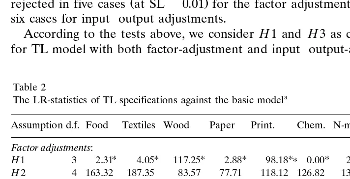
LR-statistics for the alternative hypotheses for the TL model are shown in Table
Ž .
2 the estimated parameters are not reported here to save space ; the asterisked numbers are less than the relevant critical values given in Table 1, and therefore
the corresponding hypotheses cannot be rejected at SLs0.05. The hypotheses
corresponding to the underlined and unmarked numbers are rejected at SLs0.05 and SLs0.01, respectively.
Ž .
Both H1 and H3 cannot be rejected at SLs0.05 with factor-adjustments for
Ž .
all the industries, while they are in a few cases rejected at SLs0.05 with
Ž .
inputroutput adjustments. H2, H4, and H5 are rejected at SLs0.01 in all the cases for inputroutput adjustments and most cases for factor adjustments. H6 is
Ž .
rejected in five cases at SLs0.01 for the factor adjustment specification and in six cases for inputroutput adjustments.
According to the tests above, we consider H1 and H3 as candidate hypotheses for TL model with both factor-adjustment and inputroutput-adjustment except in
Table 2
a The LR-statistics of TL specifications against the basic model
Assumption d.f. Food Textiles Wood Paper Print. Chem. N-m min. B. metal Mach. Factor adjustments:
U U U U UU U U U U
H1 3 y2.31 4.05 y117.25 2.88 y98.18 0.00 y20.74 y15.74 5.80
U
H2 4 163.32 187.35 83.57 y77.71 118.12 126.82 134.13 y94.97 157.78
U U U U U U U U U
H3 4 y3.82 5.56 y121.22 1.20 y105.54 y0.99 y25.08 y14.43 3.98
U
H4 4 61.26 89.62 43.07 52.26 55.61 41.90 y2.66 64.48 70.69
U
H5 8 56.78 118.23 57.22 46.62 55.06 42.82 7.31 61.38 70.60
U U U U
H6 8 0.93 45.12 y61.46 105.48 y86.40 58.19 27.60 53.14 y25.46 Inputroutput adjustments:
U U U U U U U
H1 3 y2.85 y64.12 y60.98 y2.44 y66.10 y2.97 10.40 y7.16 8.60 H2 4 323.65 305.49 308.10 265.85 418.92 282.86 287.68 317.82 429.99
U U U U U U U U
H3 4 y0.28 y59.31 y56.28 0.53 y102.53 0.54 y5.30 y1.97 11.84
H4 4 134.64 50.40 147.65 68.68 72.02 35.33 34.37 70.03 82.33
H5 8 132.27 ] 158.77 63.26 87.59 32.62 43.84 69.82 ]
H6 8 1.84U
63.17 87.18 95.04 ] 55.16 46.81 54.54 y18.27U
a
Table 3
Ž .
The LR test of H3 against H1 for TL model d.f.sl
Adjustment Food Textiles Wood Paper Print. Chem. N-m min. B. metal Mach. Factor y1.51 1.51 y3.96 y1.68 y7.36 y0.99 y4.34 1.31 y1.82 Inputroutput 2.57 4.81 4.70 2.97 y36.43 3.51 y15.70 5.20 3.24
the case of machinery industry, for which, we accept H6. We thus have to test H3
Ž .
against H1 with d.f.s1 for all the industries except machinery with inputr
out-Ž .
put adjustments. For the tests, we control the overall conventional SL 5% and uniformly assigned a significance level of 0.0125 to each d.f. for the testing of H3
Ž . Ž
against H1 obtaining an interpolated critical value chi-squared of 6.33 d.f.s1,
.
SLs0.0125 . The statistics for testing of H3 against H1 are shown in Table 3; all
Ž .
the statistics are less than the critical value of 6.33 d.f.s1 at the assigned significance level of 0.0125, thus we cannot reject H3 but accept it. Because a large number of coefficients of auto-correlation in the inputroutput-adjustments are larger than unity, we discard this adjustment mechanism in favor of factor-adjust-ments.
4.2. Tests of alternati¨e GL model hypotheses
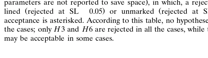
For the GL model, we test all the seven hypotheses listed above against the basic GL model at the conventional SLs0.05. The LR-statistics for the alternative
Ž
hypotheses of restricted GL models are shown in Table 4 again the estimated
.
parameters are not reported to save space , in which, a rejection is either
under-Ž . Ž .
lined rejected at SLs0.05 or unmarked rejected at SLs0.01 , while an
acceptance is asterisked. According to this table, no hypotheses are accepted in all the cases; onlyH3 and H6 are rejected in all the cases, while the other hypotheses may be acceptable in some cases.
Table 4
a Statistics for LR test of GL specifications against the basic model
Assumption d.f. Food Textiles Wood Paper Print. Chem. N-m min. B. metal Mach.
U U
H1 3 0.09 10.48 13.39 21.98 11.10 24.91 y2.98 18.21 14.58
U U
H2 4 0.10 9.82 18.57 28.72 25.33 23.34 y3.50 22.05 42.94
H3 4 49.04 49.92 63.20 94.40 29.50 92.96 15.62 37.52 48.62
U U
H4 3 y0.32 21.96 17.03 11.98 1.69 23.86 11.66 15.36 34.57
U U
H5 4 y0.24 29.71 24.44 21.46 2.00 36.27 18.07 26.83 38.91
H6 4 26.32 119.88 75.42 138.74 50.96 94.02 49.68 146.72 135.58
U U
H7 1 5.14 20.05 1.85 y3.36 14.72 11.14 9.15 6.39 32.56
aNote.
For textiles, chemicals, base metals, and machinery industries, the tests reject all the null hypotheses against the basic model.
For wood and paper industries, H7 is uniquely accepted. For the remainder of the industries, further tests were made as follows.
For the food industry, H1, H2, H4, and H5 cannot be rejected. Because H2 is nested in H1 and H5 in H4, we might use the LR-test to test H2 against H1 and
H5 against H4; because the former two and the latter two hypotheses are not
Ž
nested in each other, we might use the J-test technique Davidson and MacKinnon,
.
1981 for testing them. However, we found that each of the non-rejected specifica-tions and the basic model produced at least one negative elasticity of factor]input concerning output. Among the remainders, only H7 has produced positive elastici-ties of factors with respect to output; therefore, we use H7 for further analyses. In the case of non-metallic minerals, H1 and H2 cannot be rejected. We further tested the latter against the former and obtained the LR-statistics of 0.62 which are
Ž .
smaller than the critical values of 6.33 SLs0.0125, d.f.s1 ; therefore, we accept
H2. In this test, we also control the overall significance level at 5%.
For the printing industry, H4 and H5 cannot be rejected against the basic model as shown in Table 4, H5 is nested in H4, and therefore we can test the former
Ž .
against the latter with an LR-test. We control the overall significance level 5% in the same way. As the LR-statistic of 0.31 is smaller than the critical values of 6.33
ŽSLs0.0125, d.f.s1 we cannot reject. H5 but accept it.
By the tests, we find that the two models disagree on production technology, since the TL accepts the assumption of putty]putty production technology, while the GL rejects such an hypothesis.
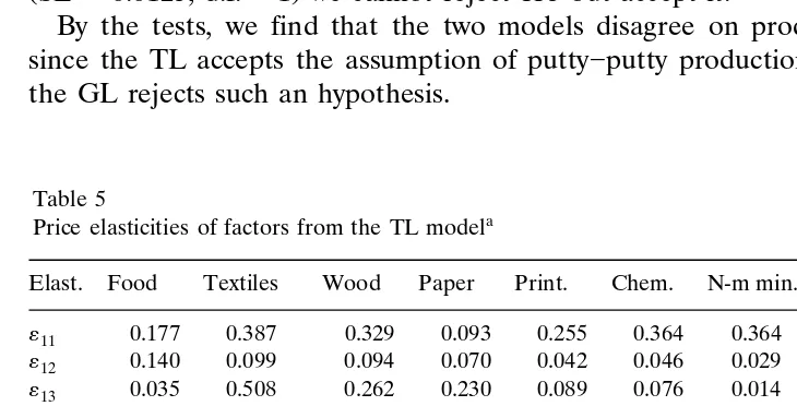
Table 5
a Price elasticities of factors from the TL model
Elast. Food Textiles Wood Paper Print. Chem. N-m min. B. metal Mach. «11 y0.177 y0.387 y0.329 0.093 y0.255 y0.364 y0.364 y0.146 y0.207 «12 y0.140 y0.099 0.094 y0.070 0.042 0.046 0.029 y0.027 y0.027 «13 y0.035 y0.508 0.262 y0.230 0.089 y0.076 0.014 0.065 y0.219
«14 0.351 0.994 y0.026 0.214 0.124 0.394 0.322 0.108 0.454
«21 y0.110 y0.078 0.136 y0.130 0.046 0.094 0.011 y0.018 y0.032 «22 y0.118 y0.388 y0.295 y0.080 y0.309 y0.230 y0.107 y0.078 y0.311
«23 0.169 0.419 y0.133 0.329 0.387 0.458 0.085 0.112 y0.042
«24 0.059 0.047 0.292 y0.110 y0.123 y0.321 0.011 y0.017 0.386 «31 y0.001 y0.010 0.011 y0.050 0.001 y0.007 0.001 0.010 y0.004
«32 0.009 0.013 0.000 0.044 0.004 0.022 0.016 0.026 0.000
«33 y0.065 y0.120 y0.136 y0.050 y0.028 y0.101 y0.120 y0.034 y0.092
«34 0.057 0.116 0.125 0.058 0.023 0.086 0.103 y0.002 0.096
«41 0.018 0.076 y0.003 0.083 0.005 0.064 0.047 0.026 0.038
«42 0.005 0.006 0.025 y0.020 y0.003 y0.024 0.007 y0.003 0.029
«43 0.077 0.404 0.327 0.101 0.094 0.148 0.228 y0.005 0.363
«44 y0.100 y0.486 y0.349 y0.170 y0.096 y0.188 y0.281 y0.019 y0.430 a
5. Price elasticities of factors and factor substitutions
This section presents the price elasticities of factors and factor substitutabilities from the TL and GL models. As the two models disagree in production technology, we expect different results of price elasticities and factor substitutabilities from them.
5.1. Price elasticities of factors from the TL model
From the TL model we obtain the same short- and long-run elasticities of inputs
Ž .
with respect to prices for all the industries see Table 5 , as the model accepts instantaneous adjustments of factors. This unexpected result could either indicate poor data or poor model in capturing a short-run production.
There is one aberration of own-price elasticity; of 36 own-price elasticities, all are negative as expected except elasticity «11 for the paper industry.
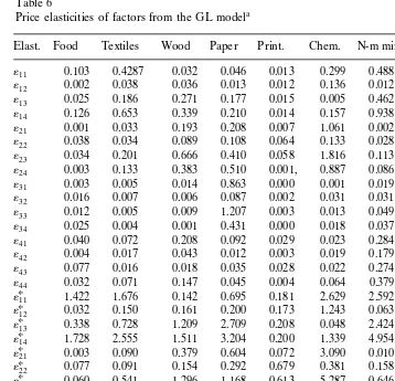
5.2. Price elasticities of factors from the GL model
In contrast to the TL model, the GL model has produced quite different short-and long-run elasticities of factors with respect to prices; the absolute values of short-run own-price elasticities of factors obtained with the GL model are
rela-Ž .
tively smaller than long-runs in all the cases of negative values see Table 6 as expected. Besides, in most of the cases, the absolute values of the short-run cross-price elasticities of factors are also quite smaller than the long-run counter-parts; this is a major difference in the comparison of the GL and TL models. These results indicate that the GL model is better suited to describing short-run produc-tion than the TL model, at least for the industries under study.
Ž .
However, one own-price elasticity both short- and long-run for electricity, five for labor and two for capital are positive. Such results are not what we expected. From this point of view, the GL model is not better for estimating own-price elasticities of factors than the GL model.
5.3. Allen elasticities of substitution
Ž . Ž .
Table 6
a Price elasticities of factors from the GL model
Elast. Food Textiles Wood Paper Print. Chem. N-m min. B. metal Mach. «11 y0.103 y0.4287 y0.032 y0.046 y0.013 y0.299 y0.488 y0.098 0.258 «12 0.002 y0.038 y0.036 0.013 0.012 0.136 0.012 y0.001 y0.167 «13 y0.025 y0.186 y0.271 y0.177 0.015 0.005 y0.462 y0.176 y0.679
«14 0.126 0.653 0.339 0.210 y0.014 0.157 0.938 0.275 0.588
«21 0.001 y0.033 y0.193 0.208 0.007 1.061 0.002 y0.001 y0.075 «22 y0.038 y0.034 y0.089 y0.108 y0.064 y0.133 y0.028 y0.137 y0.127
«23 0.034 0.201 0.666 0.410 0.058 y1.816 0.113 0.274 0.232
«24 0.003 y0.133 y0.383 y0.510 y0.001, 0.887 y0.086 y0.136 y0.029 «31 y0.003 y0.005 y0.014 y0.863 0.000 0.001 y0.019 y0.188 y0.031
«32 0.016 0.007 0.006 0.087 0.002 y0.031 0.031 0.276 0.022
«33 0.012 y0.005 0.009 1.207 y0.003 0.013 y0.049 y0.074 0.029 «34 y0.025 0.004 y0.001 y0.431 0.000 0.018 0.037 y0.014 y0.020
«41 0.040 0.072 0.208 0.092 y0.029 0.023 0.284 0.128 0.039
«42 0.004 y0.017 y0.043 y0.012 y0.003 0.019 y0.179 y0.063 y0.004
«14 1.728 2.555 1.511 3.204 y0.200 1.339 4.954 1.006 1.184
U
«21 0.003 y0.090 y0.379 0.604 0.072 3.090 0.010 y0.002 y0.343
U
«22 y0.077 y0.091 y0.154 y0.292 y0.679 y0.381 y0.158 y0.235 y0.581
U
«23 0.060 0.541 1.296 1.168 0.613 y5.287 0.646 0.469 1.058
U
«24 0.014 y0.359 y0.762 y1.481 y0.006 2.578 y0.499 y0.233 y0.134
U
«31 y0.037 y0.026 y0.121 y10.806 0.004 0.006 y0.105 y2.101 y0.024
«U32 0.220 0.032 0.055 1.113 0.033 y0.315 0.167 3.082 0.017
U
«33 0.164 y0.026 0.079 15.072 y0.041 0.141 y0.272 y0.824 0.023
U
«34 y0.347 0.020 y0.013 y5.379 0.004 0.167 0.210 y0.157 y0.016
U
«41 0.124 0.101 0.232 1.386 y0.012 0.214 1.540 0.316 0.072
U
1, electricity; 2, fuels; 3, labor; 4, capital;U
, long-run.
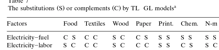
textiles, wood, non-metallic minerals, and machinery. Labor and capital substitute for each other in all industries except base metals.
Ž .
We now look at the GL-model results after slashes in Table 7 . Electricity and fuels substitute each other in food, paper, printing, chemicals, and non-metallic minerals; electricity and labor substitute only in printing and chemicals; electricity and capital substitute in all the industries except printing; labor and fuels substi-tute in all the industries except chemicals; fuels and capital substisubsti-tute in only food and chemical; labor and capital substitute in textiles, printing, chemicals, and non-metallic minerals.
Ž .
Table 7
a
Ž . Ž .
The substitutions S or complements C by TLrGL models
Factors Food Textiles Wood Paper Print. Chem. N-m min. B. metal Mach. Electricity]fuel CrS CrC SrC CrS SrS SrS SrS CrC CrC Electricity]labor SrC CrC SrC CrC SrS CrS SrC SrC CrC Electricity]capital SrS SrS CrS SrS SrC SrS SrS SrS SrS Fuel]labor SrS SrS CrS SrS SrS SrC SrS SrS CrS Fuel]capital SrS SrC SrC CrC CrC CrS SrC CrC SrC Labor]capital SrC SrS SrC SrC SrS SrS SrS CrC SrC
a
Note.A result from the TL model comes first and a result from the GL model comes after the slash.
and capital and between fuel and labor, or between electricity and fuel, in most of the industries. However, they fail to agree in the substitutabilities between electric-ity and capital in wood and printing, and between fuel and labor in wood, chemicals, and machinery, or between electricity and fuel in food, wood, and paper. For electricity]labor, fuel]capital, and labor]capital these models have produced opposite results in at least four cases. For labor and capital, the TL model suggests substitutions in all the cases except base metals, whereas the GL model shows substitutions in only textiles, printing, chemicals, and non-metallic minerals. For textiles, printing, and base metals, the two models match in substitutabilities in almost all the cases, while for wood, they generate opposite results.
6. Conclusions
The TL and GL models disagree in production technology, since the former accepts putty]putty production technology, while the latter rejects it.
There is no uniform substitution or complement between any two factors except electricity and capital. The models agree in only half of the cases. The GL model shows complement between electricity and labor, fuels and capital, and labor and capital in most of the industries, whereas the TL model shows substitution between labor and capital in most of the industries, and no obvious relationship between electricity and labor or between fuels and capital. However, both models agree that electricity and capital, or fuels and labor, can substitute for each other in most of the industries.
Both models have produced some unreasonable positive own-price factor elastic-ities: the GL model produced eight and the TL only one.
Acknowledgements
References
Ž .
Berndt, E.R., 1991. Duality and flexible functional forms. In: Berndt, E.R. Ed. , The Practice of Econometrics: Classic and Contemporary. Addison]Wesley Publishing Company, pp. 459]479. Berndt, E.R., Wood, D.O., 1975. Technology, prices, and the derived demand for energy. Rev. Econ.
Ž .
Stat. LVII 3 , 259]268.
Berndt, E.R., Fuss, M.A., Waverman, L., 1977. Dynamic Models of the Industrial Demand for Energy. EPRI EA-580. Electric Power Research Institute, Palo Alto, California
Chamberg, R.G., 1988. Applied Production Analysis: a Dual Approach. Cambridge University Press. Conrad, K., Unger, R., 1987. Ex post test for short- and long-run optimization. J. Econ. 36, 339]358. Davidson, R., MacKinnon, J.G., 1981. Several tests for model specification in the presence of alternative
Ž .
hypotheses. Econometrica 49 3 , 781]793.
Fuss, M.A., 1977. The demand for energy in Canadian manufacturing: an example of the estimation of production structures with many inputs. J. Econom. 5, 89]116.
Førsund, F.R., Hjalmarsson, L., 1987. Analyses of Industrial Structure: a Putty]Clay Approach. Almqvist & Wiksell International, Stockholm.
Gollop, F.M., Roberts, M.L., 1983. Environment regulations and productivity growth: the case of
Ž .
fossil-fueled electric power generation. J. Pol. Econ. 91 1 , 654]674.
Holly, S., Smith, P., 1986. Interrelated Factor Demanding for Manufacturing: a Dynamic Translog Cost Function Approach. Discussion Paper No. 18]86. Centre for Economic Forecasting, London Business School.
Hogan, W.W., 1989. A dynamic putty]semi-putty model of aggregate energy demand. Energy Econ. 11
Ž .1 , 53]69.
Moroney, J.R., Trapani, J.M., 1981. Alternative models of substitution and technical change in natural
Ž .
resource intensive industries. In: Berndt, E.R., Field, B.C. Eds. , Modelling and Measuring Natural Resource Substitution. MIT Press, London, pp. 48]69.
Nadiri, M.I., Rosen, S., 1969. Interrelated factor demand functions. Am. Econ. Rev. 59, 457]471. Rosen, S., Nadiri, M.I., 1974. A disequilibrium model of demand for factors of production. Am. Econ.
Ž .
Assoc. 64 2 , 264]270.
Siddayao, C.M. et al., 1987. Estimation energy and non-energy elasticities in selected Asian
manufactur-Ž .
ing sectors. Energy Econ. 9 2 , 115]128.
Tsai, D.H., Norsworthy, J.R., 1991. Productivity Growth, Technical Change, and the Structure of Production in the U.S. Machine Tool Industry. Working paper, Department of Economics and Finance, Clarkson University.
Vlachou, A.S., Samouilidis, E.J., 1986. Interfuel substitution: results from several sectors of the Greek
Ž .
economy. Energy Econ. 8 1 , 39]45.
Walfridson, B., 1985. An Ad-hoc Dynamic Energy Demand Model of the Swedish Industry Sectors. Working Paper, Department of Economics, Goteborg University.¨
Walfridson, B., 1987. Dynamic Models of Factor Demand: an Application to Swedish Industry. Doctoral Dissertation, University of Gothenburg.
Walfridson, B., 1992. Modelling Substitution and Capacity Utilisation in Dynamic Factor Demand. Working Paper, Department of Economics, Goteborg University.¨
Watkins, G.C., 1991. Short- and long-run equilibria: relationships between first and third generation
Ž .