The relationship between energy
consumption, energy prices and economic
growth: time series evidence from Asian
developing countries
qJohn Asafu-Adjaye
UDepartment of Economics, The Uni¨ersity of Queensland, Brisbane, Q4072, Australia
Abstract
This paper estimates the causal relationships between energy consumption and income for India, Indonesia, the Philippines and Thailand, using cointegration and error-correction modelling techniques. The results indicate that, in the short-run, unidirectional Granger causality runs from energy to income for India and Indonesia, while bidirectional Granger causality runs from energy to income for Thailand and the Philippines. In the case of Thailand and the Philippines, energy, income and prices are mutually causal. The study results do not support the view that energy and income are neutral with respect to each other, with the exception of Indonesia and India where neutrality is observed in the short-run.Q2000 Elsevier Science B.V. All rights reserved.
JEL classifications:C22; Q43; Q48
Keywords:Energy consumption; Economic growth; Granger causality
1. Introduction
In the past two decades numerous studies have examined the causal relation-ships between energy consumption and economic growth, with either income or
q
An earlier version of this paper was presented at the 43rd Annual Conference of the Australian Agricultural and Resource Economics Society Conference, Christchurch, New Zealand, 20]22 January 1999. Comments of conference participants and an anonymous journal reviewer are gratefully ac-knowledged. However, the usual caveat applies.
U
Fax:q61-7-3365-7299.
Ž .
E-mail address:[email protected] J. Asafu-Adjaye .
0140-9883r00r$ - see front matterQ2000 Elsevier Science B.V. All rights reserved.
Ž .
employment used as a proxy for the latter. To date, the empirical findings have been mixed or conflicting. The seminal article on this topic was published in the
Ž .
late seventies by Kraft and Kraft 1978 who found evidence in favour of causality running from GNP to energy consumption in the United States, using data for the
period 1947]1974. Their findings were later supported by other researchers. For
Ž .
example, Akarca and Long 1979 found unidirectional Granger causality running from energy consumption to employment with no feedback, using US monthly data
for the period 1973]1978. They estimated the long-run elasticity of total
employ-ment with respect to energy consumption to bey0.1356.
However, these findings have been subjected to empirical challenge. Akarca and
Ž . Ž . Ž . Ž .
Long 1980 , Erol and Yu 1987a , Yu and Choi 1985 , and Yu and Hwang 1984
Ž .
found no causal relationships between income proxied by GNP and energy consumption. On the causal relationship between energy consumption and
employ-Ž . Ž . Ž .
ment, Erol and Yu 1987b, 1989 , Yu and Jin 1992 , and Yu et al. 1988 found evidence in favour of neutrality of energy consumption with respect to employ-ment, referred to as the ‘neutrality hypothesis’.
One of the reasons for the disparate and often conflicting empirical findings on the relationship between energy consumption and economic growth lies in the variety of approaches and testing procedures employed in the analyses. Many of the earlier analyses employed simple log-linear models estimated by ordinary least
Ž .
squares OLS without any regard for the nature of the time series properties of the variables involved. However, as has recently been proven, most economic time
Ž .
series are non-stationary in levels form see Granger and Newbold, 1974 . Thus, failure to account for such properties could result in misleading relationships among the variables.
Following advances in time series analysis in the last decade, recent tests of the
energy consumption]economic growth relationship have employed bivariate
Ž . Ž .
causality procedures based on Granger 1969 and Sims’ Sims, 1972 tests. How-ever, these tests may fail to detect additional channels of causality and can also
Ž .
lead to conflicting results. For example, recently, Glasure and Lee 1997 tested for causality between energy consumption and GDP for South Korea and Singapore using the standard Granger test, as well as cointegration and error-correction modelling. They found bidirectional causality between income and energy for both countries, using cointegration and error-correction modelling. However, using the standard Granger causality tests, they found no causal relationships between GDP and energy for South Korea and unidirectional Granger causality from energy to GDP for Singapore.
The direction of causation between energy consumption and economic growth has significant policy implications. If, for example, there exists unidirectional Granger causality running from income to energy, it may be implied that energy conservation policies may be implemented with little adverse or no effects on economic growth. In the case of negative causality running from employment to
Ž .
to a fall in income or employment. The finding of no causality in either direction,
Ž .
the so-called ‘neutrality hypothesis’ Yu and Jin, 1992 , would imply that energy conservation policies do not affect economic growth.
This paper examines the energy]income relationship for four energy-dependent
Asian developing countries: India, Indonesia, the Philippines and Thailand. These countries were chosen because they represent energy-dependent LDCs which are poised for take-off into a phase of industrialisation. We depart from previous
Ž .
studies by considering a trivariate model energy, income and prices rather than the usual bivariate approach. This approach offers the opportunity to investigate other channels in the causal links between energy consumption and economic growth.
The remainder of this paper is organised in the following fashion. Section 2 presents a brief overview of the economic and energy use profiles of the countries in the sample. Sections 3 and 4 briefly describe the methodology employed and the data sources, respectively. The penultimate section presents and discusses the empirical results while the final section contains the conclusions.
2. Economic and energy use profiles
The four countries are heavily populated and have a combined total of 1.3 billion
Ž .
people Table 1 . Of the four, India is the least wealthy on a per capita income
Ž .
basis of comparison, with a per capita GDP of US$380 1996 dollars which is the average for the South Asia region. The others have per capita incomes of over
Ž .
US$1000 see Table 1 . All four countries recorded high annual growth rates in their manufacturing sectors in 1996, ranging from 10.5% for Indonesia to 5.6% for the Philippines. Of course, these impressive growth rates would have declined in 1997 and beyond in view of the Asian financial crisis. To maintain the high levels of economic output these countries make high demands on energy resources.
Table 1 reports figures for per capita energy use and carbon dioxide emissions for the four countries in the sample. Energy use per capita is highest for Thailand
Table 1
a Ž .
Per capita energy use and carbon dioxide emissions 1995
Indicator India Indonesia Thailand Philippines
Ž .
Population mid-1996 millions 945.1 197.1 60.0 71.0
Ž .
GNP per capita 1996 US$ 380 1080 2960 1160
Ž
Manufacturing average growth rate
.
% p.a. 8.1 10.5 7.7 5.6
Ž .
Energy use per capita kg 260 442 878 307
Ž .
CO emissions per capita mton2 1.0 1.5 2.9 0.9
a Ž .
in 1995 with 878 kg, followed by Indonesia with 442 kg per capita. India has the lowest per capita energy use with 260 kg. Carbon dioxide emissions per capita are also relatively high, ranging from 2.9 metric tons for Thailand to 0.9 metric tons for the Philippines. Most of the countries have to rely on imports for their energy needs, except Indonesia which is a net exporter of fuel. India is among the largest consumers of energy in the region. India’s energy sources comprise mainly coal,
Ž .
and was estimated to be 244 million metric tons in 1991 OECD, 1993 .
The above figures show that Asian LDCs account for a significant proportion of world energy consumption. Given the recent phenomenal growth in awareness of
and concern for global warming, an examination of the energy]income relationship
has implications for energy policy in these countries. It is important to add that most of the studies referred to above have dealt with advanced or newly
industri-Ž .
alised countries NICs and it may be argued that the results are not applicable to countries at a different stage of development.
3. Methodology and data
The modelling strategy adopted in this study was based on the now widely used
Ž
Engle]Granger methodology see Granger and Newbold, 1974; Engle and Granger,
. Ž . Ž .
1981 . The augmented Dicky]Fuller ADF and Phillips]Perron PP tests of
Ž .
stationarity were used Dickey and Fuller, 1981; Phillips and Perron, 1988 . Following the unit root and cointegration tests, we estimated the following error correction model:
where yt, ent, pt are real income, energy consumption and prices, respectively; D
Ž .
is a difference operator; Ai j L are polynomials in the lag operator L; ECT is the
Ž .
lagged error-correction term s derived from the long-run cointegrating
relation-ship; and the ui ts are error-correction terms assumed to be uncorrelated and
Ž .
random with mean zero. The coefficients,l isen, y, p, of the ECTs represent
i
the deviation of the dependent variables from the long-run equilibrium.
Through the error-correction mechanism, the ECM opens up an additional
Ž .
causality channel which is overlooked by the standard Granger 1969 and Sims
Ž1972 testing procedures. In the Granger sense a variable. X causes another
variableY if the current value of Y can better be predicted by using past values of
the significance of the A s conditional on the optimum lags.1 Through the ECT, i j
Ž
an error correction model offers an alternative test of causality or weak exogeneity
.
of the dependent variable . If, for example,len is zero, then it can be implied that
the change in ent does not respond to deviation in long-run equilibrium in period
ty1. Also, if l is zero and both A and A are zero, it can be implied that
en 11 13
income and prices do not Granger-cause energy consumption. The non-significance
of both the t and Wald F-statistics in the ECM will imply that the dependent
variable is weakly exogenous.2
If the variables, yt, ent and pt are cointegrated then it is expected that at least
one or all of the ECTs should be significantly non-zero. Granger causality of the
Ž . Ž .
dependent variables is tested as follows: 1 by a simple t-test of the ls; 2 by a
i
joint Wald F-test of the significance of the sum of the lags of each of the
Ž .
explanatory variables in turn; and 3 by a joint Wald F-test of the following
Ž . Ž . Ž . Ž . Ž .
interactive terms: Eq. 1 } l and A , l and A ; Eq. 2 } l and A ,
y 22 y 23 en 11
Žl and A .; and Eq. 3Ž . } Žl and A . Ž, l and A ..
en 13 p 31 p 32
Annual time series data were utilised in this study. The series for India and
Indonesia cover the period 1973]1995, while those for Thailand and the
Philip-pines cover the period 1971]1995. The data were obtained from World De¨
elop-( )
ment Indicators WDI 1998, published by the World Bank. The choice of the starting period was constrained by the availability of data on energy consumption. The precise definitions of the variables are as follows:
en: commercial energy use in kilograms of oil equivalent per capita.
y: real income, defined as GDP in constant 1987 prices in local currency units.
p: prices. Since energy prices were not available, this variable was proxied by
Ž .
the consumer price index CPI , 1987s100.
4. Empirical results and discussion
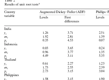
Table 2 reports the results for both the ADF and PP test results. It can be seen that, with exception of Indonesian prices, the null hypothesis of nonstationarity cannot be rejected at the 10% level for the levels of the variables. However, when first differences are taken, the null hypothesis of nonstationarity is rejected for most of the variables. We have mixed results for the differenced Thailand energy and income variables. The null hypothesis of non-stationarity cannot be rejected by the ADF test but is rejected by the PP test. It can therefore be concluded that in
Ž .
most cases, income, energy and prices are integrated of order one, that is, I 1 , except Thailand energy and income which could be integrated of order two.
1
The lag lengths were assigned on the basis of minimising Akaike’s AIC criterion.
2 Ž .
Table 2
a Results of unit root tests
Ž . Ž .
Countryr Augmented Dickey]Fuller ADF Phillips]Perron PP
variable Levels First Levels First
differences differences
Note: The optimal lags for the ADF tests were selected based on optimising Akaike’s Information
Ž .
Criteria AIC , using a range of lags. Truncation lags for the PP test were determined using the highest significant lag from either the autocorrelation or partial autocorrelation function of the first differenced series.
Given that most of the variables are integrated of the same order, the next step was to test for cointegration using Johansen’s multivariate maximum likelihood
procedure.3 The test results are reported in Table 3, where r represents the
number of cointegrating vectors. It can be seen that, for India, the null hypothesis of no cointegration relationships is rejected against the alternative of one cointe-grating relationship at the 1% level. In the case of Indonesia, the test results suggest the presence of two cointegrating relationships. Finally, the results for Thailand and the Philippines suggest that, in both cases, the null hypothesis of no cointegrating relationship can be rejected in favour of the alternative of a single
cointegrating relationship.4 The existence of cointegrating relationships among
income, energy and prices suggests that there must be Granger causality in at least
3 Ž .
The Johansen approach Johansen, 1988; Johansen and Juselius, 1990 has been shown to be superior to Engle and Granger’s residual-based approach. Among other things, the Johansen approach is capable of detecting multiple cointegrating relationships.
4
Table 3
Ž
Results of Johansen’s maximum likelihood tests for multiple cointegrating relationships intercept, no
.
trend
Countryrnull Characteristic Test 5% Critical 1% Critical
a
hypothesis roots statistics value value
India
The test statistic is thel value. Significant at theUUU
1% level, theUU
5% level and theU
10% ma x
level.
one direction. However, it does not indicate the direction of temporal causality between the variables. To determine the direction of causation, we must examine the ECM results.
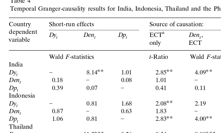
In addition to providing an indication of the direction of causality, the ECM enables us to distinguish between ‘short-run’ and ‘long-run’ Granger causality. In
Table 4, we provide joint Wald F-statistics of the lagged explanatory variables of
the ECM. These tests give an indication of the significance of short-run causal
effects. We also provide t-statistics for the coefficients of the ECTs which give an
indication of long-run causal effects. Finally, we provide joint Wald F-statistics for
Ž .
the interactive terms i.e. the ECTs and the explanatory variables which give an
indication of which variables bear the burden of short-run adjustment to re-estab-lish long-run equilibrium, given a shock to the system.
Ž .
Turning first to the short-run results for India Table 4 , it can be seen that the
Ž .
F-statistic for energy in the income equation is significant at the 5% level. However, none of the lagged explanatory variables in the other two equations
Ženergy and price are statistically significant. These results imply that, in the short.
run, there is unidirectional Granger causality running from energy consumption to income, while price has a neutral effect on both energy and income. Looking at the t-statistics, it can be seen that the coefficient of ECT is significant in the income equation but is not significant in either the energy or price equation. This result can be interpreted as follows. Given a deviation of income from the long-run
Table 4
Temporal Granger-causality results for India, Indonesia, Thailand and the Philippines Countryr Short-run effects Source of causation:
dependent a
Dyt Dent Dpt ECT Dent, Dpt, Dyt,
variable only ECT ECT ECT
WaldF-statistics t-Ratio WaldF-statistics India
ECT-error correction term in the error-correction model. Significance at the UUU
1% level, the
UU
5% level and theU
10% level.
interact in a dynamic fashion to restore long-run equilibrium. However, the
non-significance of the F-statistics for price indicates it is exogenous in the system,
implying that energy consumption bears the burden of the short-term adjustment
to long-term equilibrium. The Wald F-test results in the last three columns of
Table 4 suggest that, in the long run, both energy and price Granger-cause income. The results for Indonesia are not much different from those of India. The standard Granger tests would have concluded that there are no causal relationships
among yt, ent and pt. However, the coefficient of ECT in the energy equation is
observe Granger causality running from energy and prices to income in both the short and long runs, with reverse causality running from energy to income.
Ž .
Our results are consistent with the findings of Masih and Masih 1997 , Hwang
Ž . Ž .
and Gum 1992 and Glasure and Lee 1997 who found evidence of bidirectional causality between income and energy for South Korea and Taiwan. However, they refute the neutrality hypothesis advanced in respect of the United States for the
Ž .
energy]income relationship Erol and Yu, 1989; Yu and Jin, 1992 in three out of
four cases. It is only in the case of Indonesia and India where neutrality between energy and income is observed in the short run. However, this can be expected in the case of Indonesia since it is a net energy exporter and therefore can be shielded from energy shocks.
The ECMs displayed reasonable goodness-of-fit based on the R2and F statistics
Žnot reported here and passed most of the diagnostic tests including the Godfrey.
LM test for serial correlation, the Engle test for first-order autoregressive
het-w Ž .x
eroscedasticity ARCH 1 , the Bera]Jacque test for normality and the Ramsey
ŽRESET test for model misspecification..
5. Conclusion
The purpose of this study was to test for Granger causality between energy consumption and income for four Asian developing countries, including price as a third variable. Maximum likelihood procedures were used to analyse the time series properties of the variables and error-correction models were estimated and used to test for the direction of Granger causality. From the test results, we conclude that unidirectional Granger causality runs from energy to income for India and Indonesia, while bidirectional Granger causality runs from energy to income for Thailand and the Philippines. In the long run, there is unidirectional Granger causality running from energy and prices to income for India and Indonesia. However, in the case of Thailand and the Philippines, energy, income and prices are mutually causal. Price effects are relatively less significant in the causal chain. In general, the study results do not support the view that energy and income are neutral with respect to each other, with the exception of Indonesia and India where neutrality is observed in the short run.
The study finding of bidirectional Granger causality or feedback between energy consumption and income has a number of implications for policy analysts and forecasters. A high level of economic growth leads to high level of energy demand and vice versa. In order not to adversely affect economic growth, energy conserva-tion policies that aim at curtailing energy use must rather find ways of reducing consumer demand. Such a policy could be achieved through an appropriate mix of energy taxes and subsidies. At the same time, efforts must be made to encourage industry to adopt technology that minimises pollution.
conduct-ing econometric forecasts. Our results suggest that in some cases, energy consump-tion, income and price are endogenous and therefore single equation forecasts of one or the other could be misleading. In particular, any analysis which does not incorporate the error-correction terms is likely to give unreliable results. Our findings are consistent with the expectation that energy-dependent economies are relatively more vulnerable to energy shocks. Indonesia is the only net energy exporter in the sample and therefore we find short-run neutrality between energy and income. Thus, in the case of Indonesia, there is relatively more scope for more drastic energy conservation measures without severe impacts on economic growth.
References
Akarca, A.T., Long, T.V., 1979. Energy and employment: a time series analysis of the causal relatonship. Resources Energy 2, 151]162.
Akarca, A.T., Long, T.V., 1980. On the relationship between energy and GNP: a re-examination. J. Energy Dev. 5, 326]331.
Dickey, D.A., Fuller, W.A., 1981. Likelihood ratio statistics for autoregressive time series with a unit root. Econometrica 49, 1057]1072.
Engle, R.E., Granger, C.W.J., 1981. Cointegration and error-correction: representation, estimation and testing. Econometrica 55, 251]276.
Engle, R., Hendry, D.F., Richard, J.F., 1983. Exogeneity. Econometrica 51, 277]304.
Erol, U., Yu, E.S.H., 1987a. Time series analysis of the causal relationships between US energy and employment. Resources Energy 9, 75]89.
Erol, U., Yu, E.S.H., 1987b. On the causal relationship between energy and income for industraialised countries. J. Energy Dev. 13, 113]122.
Erol, U., Yu, E.S.H., 1989. Spectral analysis of the relationship between energy and income for industrialised countries. J. Energy Dev. 13, 113]122.
Glasure, Y.U., Lee, A.R., 1997. Cointegration, error-correction, and the relationship between GDP and energy: the case of South Korea and Singapore. Resource Energy Econ. 20, 17]25.
Granger, C., Newbold, P., 1974. Spurious regressions in econometrics. J. Econometrics 2, 111]120. Granger, C.W.J., 1969. Investigating causal relations by econometric models and cross spectral methods.
Econometrica 37, 424]438.
Hwang, D., Gum, B., 1992. The causal relationship between energy and GNP: the case of Taiwan. J. Energy Dev. Spring, 219]226.
Johansen, S., Juselius, K., 1990. Maximum likelihood estimation and inferences on cointegration with approach. Oxford Bull. Econ. Stat. May, 169]209.
Johansen, S., 1988. Statistical analysis of cointegrating vectors. J. Econ. Dyn. Control JunerSeptember, 231]254.
Kraft, J., Kraft, A., 1978. On the relationship between energy and GNP. J. Energy Dev. 3, 401]403. Masih, A.M.M., Masih, R., 1997. On the temporal causal relationship between energy consumption, real
income and prices: some new evidence from Asian energy dependent NICs based on a multivariate cointegrationrerror-correction approach. J. Policy Modelling 19, 17]440.
OECD, 1993. Energy Statistics and Balances of Non-OECD Countries, 1990]91. OECD, Paris. Phillips, P.C.B., Perron, P., 1988. Testing for a unit root. Biometrica 75, 335]346.
Sims, C.A., 1972. Money, income and causality. Am. Econ. Rev. 62, 540]552.
World Bank, 1998. World Development Indicators 1998, CD ROM version. Washington, DC. Yu, E.S.H., Choi, J.Y., 1985. The causal relationship between energy and GNP: an international
Yu, E.S.H., Hwang, B.K., 1984. The relationship between energy and GNP: further results. Energy Econ. 6, 186]190.
Yu, E.S.H., Jin, J.C., 1992. Cointegration tests of energy consumption, income and employment. Resources Energy 14, 259]266.