MONITORING OF FLUVIAL TRANSPORT IN THE MOUNTAIN RIVER BED USING
TERRESTRIAL LASER SCANNING
G. Jozkow a, *, A. Borkowski a, M. Kasprzak b a
Institute of Geodesy and Geoinformatics, Wroclaw University of Environmental and Life Sciences, Grunwaldzka 53, 50-357 Wroclaw, Poland - (grzegorz.jozkow, andrzej.borkowski)@igig.up.wroc.pl b
Institute of Geography and Regional Development, University of Wroclaw, pl. Uniwersytecki 1, 50-137 Wroclaw, Poland - marek.kasprzak@uni.wroc.pl
Commission VII, WG VII/5
KEY WORDS: Terrestrial Laser Scanning, Monitoring, Fluvial Geomorphology, Mountain River, Sudetes
ABSTRACT:
The fluvial transport is the surface process that has a strong impact on the topography changes, especially in mountain areas. Traditional hydrological measurements usually give a good understanding of the river flow, however, the information of the bedload movement in the rivers is still insufficient. In particular, there is limited knowledge about the movement of the largest clasts, i.e. boulders. This investigation addresses mentioned issues by employing Terrestrial Laser Scanning (TLS) to monitor annual changes of the mountain river bed. The vertical changes were estimated based on the Digital Elevation Model (DEM) of difference (DoD) while transported boulders were identified based on the distances between point clouds and RGB-coloured points. Combined RGB point clouds allowed also to measure 3D displacements of boulders. The results showed that the highest dynamic of the fluvial process occurred between years 2012-2013. Obtained DoD clearly indicated alternating zones of erosion and deposition of the sediment finer fractions in the local sedimentary traps. The horizontal displacement of the rock material in the river bed showed high complexity resulting in the displacement of large boulders (major axis about 0.8 m) for the distance up to 2.3 m.
* Corresponding author
1. INTRODUCTION
The fluvial transport is the surface process that has a strong impact on the topography changes, especially in mountain areas. Advancing the knowledge of this process contributes in the understanding of surface relief formation and allows to predict its future changes. In addition, fluvial processes are related with the flood hazards what implies practical importance of studies related with fluvial geomorphology.
The traditional hydrological measurements usually give a good understanding of the river flow, however, the information of the bedload movement in the rivers is still insufficient. The data acquired using sedimentary traps provide only partial information about the fluvial transport, because it applies only to the finest fraction of the rock material. The knowledge of the fluvial transport of the largest clats, e.g. boulders (size over 256 mm) and cobbles (64-256 mm) (Wenworth, 1922) is limited because the deposition time of this fraction is long and the frequency of the hydrological incidents strong enough for its transport is low. For that reason, other techniques that provide reliable information about the movement of boulders and cobbles are desired. The remote sensing techniques can be potentially used in the fluvial transport monitoring studies since they are able to gather data at different scales.
The investigations on the fluvial transport monitoring with the use of remote sensing techniques are mainly focused on the determination of the river channel topography and its dynamic changes. Recent studies employ Terrestrial Laser Scanning (TLS) (Brasington et al., 2012; Heritage & Hetherington, 2007;
Picco et al., 2013; Williams et al., 2011; Williams et al., 2015) or Mobile Laser Scanning (MLS) (Alho et al., 2009; Brasington et al., 2012) since it can provide data at sufficient range, density, and accuracy. Obtained point clouds allow to create the model of the river bed surface, and subsequently, to estimate parameters (e.g. roughness) (Baewert et al., 2014) that impact fluvial transport. However, the goal of using TLS in such studies is the monitoring of the river bed changes, either short-term (Picco et al., 2013; Williams et al., 2011) or long-short-term (Kuo et al., 2015). These changes are determined based on the Digital Elevation Models (DEMs) created from the data acquired periodically, and consequently, on the DEM of difference (DoD) between two analysed scanning epochs. Although DoD can show accumulation and erosion zones providing quantitative values for the gravel volumes, its use is limited. The DoD does not allow to distinguish between different fractions of transported rock material what is important because different clasts are transported in different manner and for various distances. The range of transportation along the river channel or any other 2D or 3D direction cannot also be estimated based on DoD.
In this study the TLS was employed to monitor annual changes of the mountain river bed. Besides using DoDs for the estimation of bedload vertical changes, TLS point clouds were used to identify transported boulders and cobbles, and consequently, to measure 3D vectors of their displacement. The International Archives of the Photogrammetry, Remote Sensing and Spatial Information Sciences, Volume XLI-B7, 2016
2. METHODOLOGY
2.1 Vertical Changes
The method used in this study to monitor vertical changes is based on DoD. This approach is commonly used in fluvial geomorphology studies (Kuo et al., 2015). The simplest approach assumes that both DEMs are GRID type and have identical position, number and size of cells. Therefore, DoDt1-t2 is created by simple subtraction of DEMt1 from DEMt2 heights in corresponding GRID nodes. In practice, creating appropriate differential model may be more complicated because of few reasons. For example, the lack of points in occluded areas requires an interpolation that may result in improper DEMs. DEMs are 2.5D and cannot accurately describe 3D surface of irregularly shaped boulders, however, such simplification is required by DoD. The first issue was solved by creating DEMs as TIN models with excluded long edges. This resulted in DoD that has also excluded areas corresponding to occluded areas in any of source DEMs (Figure 1). For the visualisation purposes, the DoD was projected over the orthoimage where small (insignificant) DoD values (less than 1 cm in absolute terms) were set to transparent (Figure 1). Resultant DoD (Figure 1) clearly indicates accumulation and erosion zones and allows for quantitative analysis, however, it does not allow to analyze the granularity of transported clasts or the fluvial transport along horizontal direction.
Figure 1. Example of created DoD
2.2 3D Displacement of Single Boulders
The DoD can be potentially used in the detection of transported boulders or cobbles by finding positive and negative DoD areas that correspond to the same stone. Although the detection of stones moved to new place (positive values of DoD) seems to be easy (see Figure 1), the identification of the places from where the stones were removed (negative values of DoD) are more difficult. The reason is that smaller fractions need more time to settle near to newly placed boulder, but they can easily fill the gap created after large stone removal. For that reason,
the computation of the differences between two scanning epochs was executed not on the DEMs but on the point clouds. There were calculated distances between two point clouds using CloudCompare software (Girardeau-Montaut, 2016). The algorithm implemented in this software computes distances to all points contained in compared cloud with respect to points contained in reference cloud. This explains why two sets of distances for the period t1-t2 were calculated, where each point cloud was once the reference and once the compared cloud (Figure 2). If the point cloud t2 is set to reference, large distances identify old stones that were present only at the epoch t1 (Figure 2a). If the point cloud t1 is set to reference, large distances identify new stones that appeared at the epoch t2 (Figure 2b). Some significant distances between point clouds may appear as a result of the occlusion removal caused by the removal of another boulder. Obviously, such changes are not related with the fluvial transport.
(a) (b)
Figure 2. Example of distances between clouds t1 and t2 (description in the text); blue colour indicates zero distance
Figure 3. RGB point cloud combination and measurement of boulder displacement
The automatic estimation of translation and rotation parameters of moved boulders is very difficult because of two main reasons: (1) ambiguities in the identification of the same boulder, and (2) changes in the boulder size and shape. The identification of the same boulder at two different epochs that allows to perform automatic 3D or even 2D matching may be The International Archives of the Photogrammetry, Remote Sensing and Spatial Information Sciences, Volume XLI-B7, 2016
impossible due to lack of the overlap. The boulder may roll causing that various surfaces of the same stone are scanned at various epochs. In addition, water erosion in the mountain river is strong what can significantly change the shape and the texture of stones making the automatic matching extremely challenging.
The identification of the same boulders and cobbles at two different epochs, as well as the identification of new and old stones moved in and out from the test area, respectively, were performed in this study manually. The basis for the horizontal change detection were distances between point clouds (Figure 2). Since these distances are insufficient to identify the same, but moved stone, a combined point cloud with the RGB information was used for that purpose (Figure 3). In addition, this approach allowed to measure dominant axis of transported stones, and consequently, to measure 3D displacement vector (Figure 3). Such method, though manual, allowed to identify and remove possible false stone identifications due to occlusion removal. by several reasons. First, the bed of mountain streams contains large portion of the biggest fraction of the rock material that allows to collect sufficient amount of test data. Second, in the autumn season the water level in Sudeten rivers is usually very low what significantly minimizes the issues related with scanning the river bed through the water. Finally, the fluvial transport in the Sudeten is insufficiently recognized, therefore, collected data may bring new valuable information for the geomorphologists.
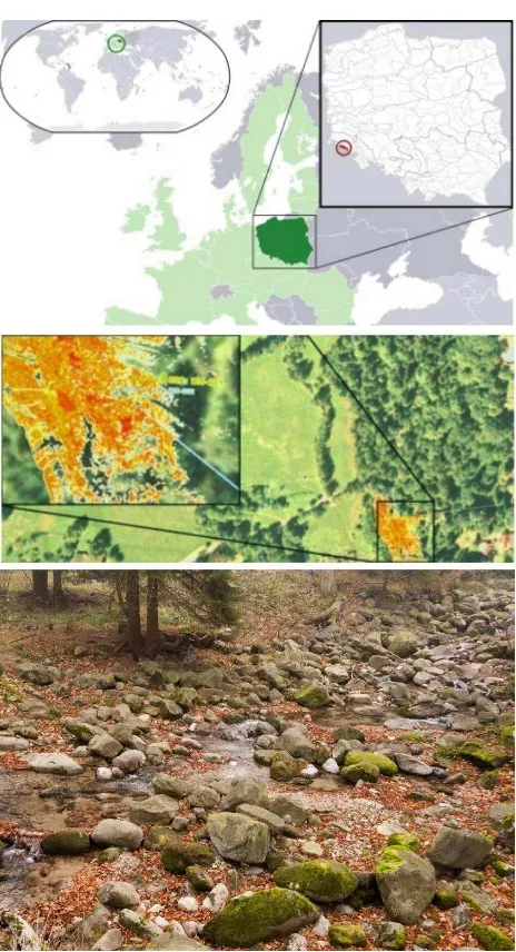
Since the Lomniczka River is typical, medium size stream of the highest Sudeten region, it was chosen as the test object in this study. The 30 m long section of this river was selected for detailed investigation and TLS data acquisition (Figure 4). This
section is characterized by steep slope over 133 ‰ for channel
longitudinal section. In addition, the topography, in particular high scarps on the river sides, allowed to select appropriate position for the scanner resulting in a close distance to the river (few meters) and larger scanning angle with respect to terrain surface that reduced the occlusion effect. One scanning position was established at each end of selected section to collect points from opposite directions.
3.2 Equipment
The test data was acquired with the pulsed, green-wavelength Leica ScanStation C10 laser scanner. The most important parameters of this scanner, including accuracy, are presented in Table 1. Since the green-wavelength is less absorbed by water, it is possible, to some extent, to obtain reflections from covered by water part of river bed. Target acquisition standard deviation 2 mm
Table 1. Leica ScanStation C10 selected parameters
3.3 Scanning Through the Water
Despite the fact that the green-wavelength is less absorbed by water, the aspect of performing the scanning through two different medias (air and water) should be discussed in more details. Obviously, the water surface refracts and/or reflects the laser beam. Such refraction results in the longer range that is measured by the scanner, and consequently, distorts coordinates of measured points. The amount of this distortion depends, among others, on two factors: scanning incidence angle and water depth. This distortion can be modelled, and appropriate corrections to point coordinates can be calculated and applied (Smith et al., 2012). However, the models are usually created The International Archives of the Photogrammetry, Remote Sensing and Spatial Information Sciences, Volume XLI-B7, 2016
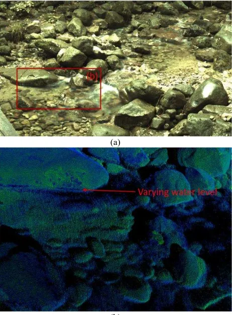
with some assumptions (e.g. flat surface of the water, constant refractive index). This causes that such models are inadequate for turbulent water flow, such as in the mountain streams, because the incident angle and water level are changing over scanning time. Figure 5a shows the example of the panorama photo taken by the scanner presenting the dynamic of the water flow as the blurry part of the image. Figure 5b shows the part of the corresponding point cloud clearly indicating higher noise for the areas scanned through the water.
(a)
(b)
Figure 5. Scanning through the water: (a) turbulent water flow, (b) noisy point cloud
Since this investigation focuses on the largest fraction of the lag deposit (boulders over 256 mm), and the test data was acquired during the low water level, the major part of the test data was
The scanning was performed annually during the autumn in the years 2011-2014. The parameters of the scanning were almost identical for each campaign, including:
similar positions of the scanner (at marked points) with similar instrument height,
identical position of warp points and scanning targets, similar scanning FOVs covering selected river
section,
the same scanning resolution with the point spacing of 3 mm at 10 m scanning range.
In addition to the laser scanning data, Leica ScanStation C10 instrument acquired RGB images used to assign the RGB information to each laser point.
Acquired data was pre-processed to register clouds collected from two scanning positions and to add the georeference to combined cloud. Both tasks were performed in the vendor provided software (Leica Cyclone Register) based on 3 scanning targets placed over the warp points with known coordinates. Note that TLS was performed with levelled scanner what adds additional constrains to the registration and georeferencing processes, and consequently, reduces number of necessary targets to 2. The point clouds were co-registered with 3D mean absolute error (MAE) equal 1-2 mm depending on the campaign. This proves the high internal accuracy of performed scanning. The accuracy of georeferencing was slightly lower with the MAE equal 2-6 mm. However, in absolute terms, such error is very small since it corresponds to the accuracy of the precise total station measurements and is significantly more accurate than GPS-RTK surveys executed to calculate absolute coordinates of warp points. To avoid possible georeferencing uncertainties, registered at different epochs point clouds were adjusted using Iterative Closest Point (ICP) algorithm. Except first epoch, each of the next epochs was matched to the previous epoch resulting in the fine adjustment of all points to the same coordinate system. Because scanned scenario changes over time, the ordinary ICP may be affected by outliers. To avoid the influence of such points, an ICP algorithm with outliers removal was used (Girardeau-Montaut, 2016). The ICP fine adjustment resulted with the internal accuracy estimate better than 1 mm for all point clouds. The results of ICP proved the high accuracy of the point cloud registration and georeferencing using three targets; the ICP resultant rotation matrices were close to identity and translation vector was smaller than 1 cm for each component.
4. RESULTS
The results of annual vertical differences are shown in Figure 6. The DoDs clearly show the accumulation (positive values) and erosion (negative values) zones for each period. The high dynamic of the fluvial transport in the mountain river bed is indicated by zones that can be the erosion zone in one period to become accumulation zone in another period. The highest dynamic was observed for the period 2012-2013 (Figure 6b). In addition to annual changes, Figure 7 shows the total vertical change over 3 years ranging from – 30 to + 30 cm. These values are much higher than the accuracy of point clouds and created models proving that fluvial transport in mountain rivers can be easily detected and quantitatively assessed using TLS data.
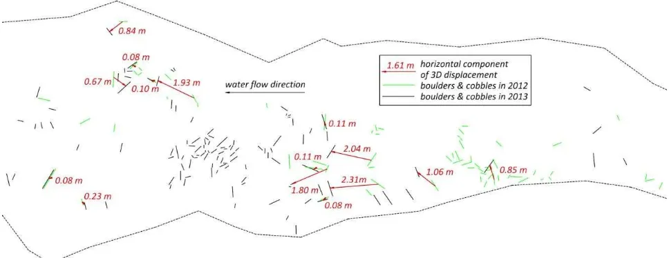
The results of the horizontal displacement between years 2012-2013 are shown in Figure 8. In addition, Figure 8 shows the river is proven additionally by different displacement directions that may occur even across the nominal flow of the stream. The International Archives of the Photogrammetry, Remote Sensing and Spatial Information Sciences, Volume XLI-B7, 2016
(a)
(b)
(c)
Figure 6. DoD for years: (a) 2012-2011, (b) 2013-2012, (c) 2014-2013 projected over orthoimage; insignificant height differences are transparent
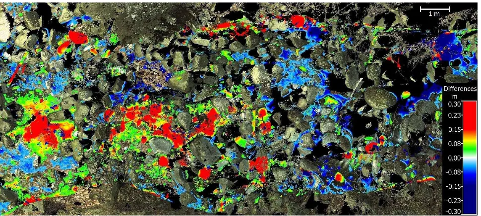
Figure 7. DoD for years 2014-2011 projected over orthoimage; insignificant height differences are transparent The International Archives of the Photogrammetry, Remote Sensing and Spatial Information Sciences, Volume XLI-B7, 2016
Figure 8. Horizontal displacements and map of moved boulders and cobbles for years 2012-2013
5. CONCLUSIONS
This investigation showed the application of TLS for the fluvial transport monitoring in the mountain river. The main goal of this study was to assess the mobility of the boulders (the largest fraction of the lag deposit) along the river channel.
The analysis executed on the point clouds and DEMs created form TLS data acquired annually during four year period allowed to asses vertical and 3D changes in the river bed caused by the fluvial transport. Created DoDs indicated accumulation and erosion zones where the absolute change of the river bed height was up to 0.4 m. The estimation of boulder 3D displacements was executed manually based on the distances between two point clouds and combined point cloud with added RGB information. Obtained results showed that the highest dynamic occurred in the period 2012-2013 where large boulders of the size 0.8 m were transported by the river for a distance about 2.3 m. Executed investigation proved that TLS can be used for the fluvial transport monitoring in the mountain river bed along vertical and horizontal directions, providing reliable information for the geomorphologists.
REFERENCES
Alho, P., Kukko, A., Hyyppä, H., Kaartinen, H., Hyyppä J., and
Jaakkola, A., 2009, Letters to ESEX. Application of boat-based laser scanning for river survey. Earth Surface Processes and Landforms, 34, pp. 1831–1838.
Baewert, H., Bimböse, M., Bryk, A., Rascher, E., Schmidt, K-H., and Morche, D., 2014. Roughness determination of coarse grained alpine river bed surfaces using Terrestrial Laser Scanning data. Zeitschriftfür Geomorphologie, Supplementary Issues, 58 (1), pp. 81-95.
Brasington, J., Vericat, D., and Rychkov, I., 2012., Modeling river bed morphology, roughness, and surface sedimentology using high resolution terrestrial laser scanning. Water Resources Research, 48 (11), 18 pages.
Girardeau-Montaut, D., 2016. CloudCompare - Open Source project. Online: http://www.danielgm.net/cc/ (accessed 30.03.2016).
Heritage, G., & Hetherington, D., 2007. Towards a protocol for laser scanning in fluvial geomorphology. Earth Surface Processes and Landforms, 32, pp. 66–74.
Kuo, Ch-W., Brierley, G., and Chang, Y-H., 2015. Monitoring channel responses to flood events of low to moderate magnitudes in a bedrock-dominated river using morphological budgeting by terrestrial laser scanning. Geomorphology, 235 (2015), pp. 1–14.
Picco, L., Mao, L., Cavalli, M., Buzzi, E., Rainato, R., and Lenzi, M.A., 2013. Evaluating short-term morphological changes in a gravel-bed braided river using terrestrial laser scanner. Geomorphology, 201, pp. 323–334.
Smith, M., Vericat, D., and Gibbins, C., 2012. Through-water terrestrial laser scanning of gravel beds at the patch scale. Earth Surface Processes and Landforms, 37, pp. 411–421.
Wentworth, C.K., 1922. A scale of grade and class terms for clastic sediments. The Journal of Geology, 30(5), pp. 377-392.
Williams, R., Brasington J., Vericat D., Hicks M., Labrosse F., and Neal, M., 2011. Monitoring Braided River Change Using Terrestrial Laser Scanning and Optical Bathymetric Mapping. Developments in Earth Surface Processes, 15, pp. 507–532.
Williams, R., Rennie, C., Brasington, J., Hicks, M., and Vericat, D., 2015. Linking the spatial distribution of bed load transport to morphological change during high-flow events in a shallow braided river. Journal of Geophysical Research, 120, pp. 604-622.