GEOLOGICAL MAPPING USING MACHINE LEARNING ALGORITHMS
A.S. Harvey a, *, G. Fotopoulos a
aQueen’s University, Department of Geological Sciences and Geological Engineering, 36 Union Street, Kingston, Ontario, Canada, K7L3N6 - (8ash5, gf26)@queensu.ca
Commission VIII, WG VIII/5
KEY WORDS: Geology, Geological Mapping, MLA, Random Forest, Spectral Imagery, Rocks
ABSTRACT:
Remotely sensed spectral imagery, geophysical (magnetic and gravity), and geodetic (elevation) data are useful in a variety of Earth science applications such as environmental monitoring and mineral exploration. Using these data with Machine Learning Algorithms (MLA), which are widely used in image analysis and statistical pattern recognition applications, may enhance preliminary geological mapping and interpretation. This approach contributes towards a rapid and objective means of geological mapping in contrast to conventional field expedition techniques. In this study, four supervised MLAs (naïve Bayes, k-nearest neighbour, random forest, and support vector machines) are compared in order to assess their performance for correctly identifying geological rocktypes in an area with complete ground validation information. Geological maps of the Sudbury region are used for calibration and validation. Percent of correct classifications was used as indicators of performance. Results show that random forest is the best approach. As expected, MLA performance improves with more calibration clusters, i.e. a more uniform distribution of calibration data over the study region. Performance is generally low, though geological trends that correspond to a ground validation map are visualized. Low performance may be the result of poor spectral images of bare rock which can be covered by vegetation or water. The distribution of calibration clusters and MLA input parameters affect the performance of the MLAs. Generally, performance improves with more uniform sampling, though this increases required computational effort and time. With the achievable performance levels in this study, the technique is useful in identifying regions of interest and identifying general rocktype trends. In particular, phase I geological site investigations will benefit from this approach and lead to the selection of sites for advanced surveys.
1. INTRODUCTION
There are many applications of remotely sensed imagery in Earth science applications such as environmental monitoring (Munyati, 2000), land use (Yuan et al., 2005), and mineral exploration (Hewson et al., 2006; Sabins, 1999). Improving exploration techniques and lithological identification in remote areas is important for improving our understanding of regional geology. Remotely sensed data has been shown to be useful for geological mapping of alteration minerals and rocktypes (Massironi et al., 2008; Rowan and Mars, 2003). As the volume and variety of data become increasingly available and useful, new obstacles arise, namely (1) manual interpretation cannot maintain the pace with the amount of incoming data and (2) manual photo interpretation is generally subjective and can be inconsistent among interpreters, especially with large datasets. This can be true for experts as well, as demonstrated in the Bond et al. (2007) study of conceptual uncertainty. Machine learning algorithms (MLA) are a rapid and more objective approach to photo interpretation that automates feature classification for these datasets – a commonly used technique in image analysis.
In Cracknell and Reading (2014) the use of MLAs in rocktype classification using remote sensed spectral imagery and geophysical datasets are assessed. It was found that some MLAs,
study because it has been reliably mapped geologically over the years.
2. BACKGROUND
2.1 Geology of the Sudbury Structure
The structure is located near where the Superior Province, the Southern Province, and the Grenville Province meet. Three main components make up the geology as follows:
1. The Sudbury Breccia, found throughout the Archean basement and surrounding Proterozoic cover.
2. The Sudbury Basin, which contains the Whitewater Group, which is composed of three Formations: (i) the Onaping Formation composed by volcanic and metasedimentary rocks; (ii) the Onwatin Formation composed of laminated mudstone and slate; and (iii) the
Chelmsford Formation, which is composed of a sequence of graded and massive wackes.
3. The Sudbury Igneous Complex (SIC), which is a lopolith structure sitting in the Sudbury Basin that is noritic and granophyric in composition. The base of this complex is associated with the Ni-Cu-PGE sulphide ores that are of economic interest.
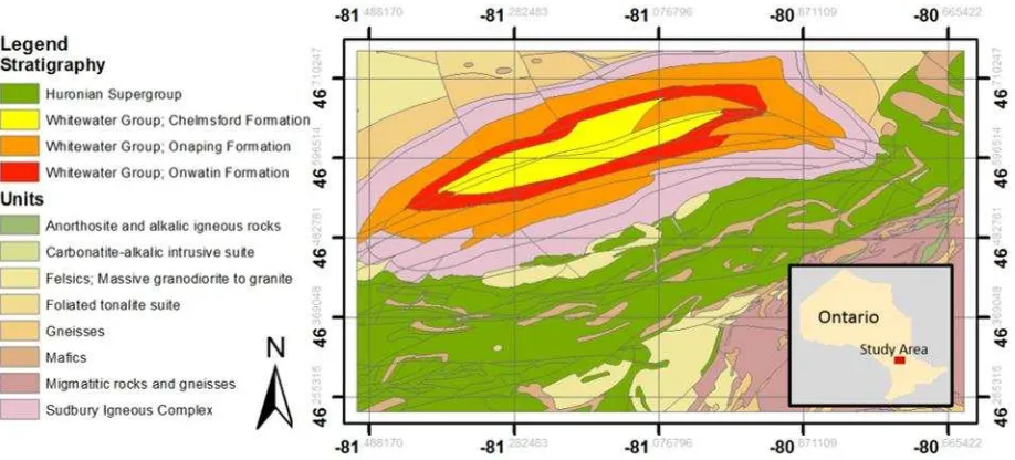
The basin is surrounded by migmatized high grade gneisses to the north and east, metavolcanic and metasedimentary rocks of the Huronian Supergroup to the south, high grade metamorphic gneisses of the Grenville Province to the southeast, and felsic plutons to the west (Peredery, 1991). The study area can be seen in Figure 1 along with major stratigraphy groups and other major rock units. A summary of dataset inputs, sources, units, and original resolutions is available in Table 1.
Figure 1. Map showing major stratigraphy groups and other major units in the Sudbury region (Ontario Geological Survey, 2011).
Feature Source and Filename Units Original Resolution
Landsat 4-5 TM Bands 1-7 October 2011
USGS
LT50190282011278EDC00
Spectral Response
16-bit data 30 m × 30 m
Digital Elevation Model
USGS; SRTM n46_w081_1arc_v3 n46_w081_1arc_v3
metres 30 m × 30 m
Total Magnetic Intensity OGS; MNDM ONMAGONL
from GDS1036 nanoTelsa 200 m × 200 m
Bouguer Gravity Anomaly OGS; MNDM ONGRAVTY1 milliGal 1000 m × 1000 m
Bedrock Geology OGS
Geopoly from MRD126-REV1 Discrete Geological Units Resampled to study area density
3. METHODOLOGY
3.1 Pre-Processing and Data Sources
Datasets in Table 1 were transformed to refer to a common datum, NAD83 and resampled to the resolution of the coarsest dataset, 1000 m × 1000 m. Spectral imagery of the region of interest was obtained from Landsat 4-5 TM datasets available from the USGS. The images were taken in October of 2011, with less seasonal vegetation cover that could obstruct the imagery. Various band
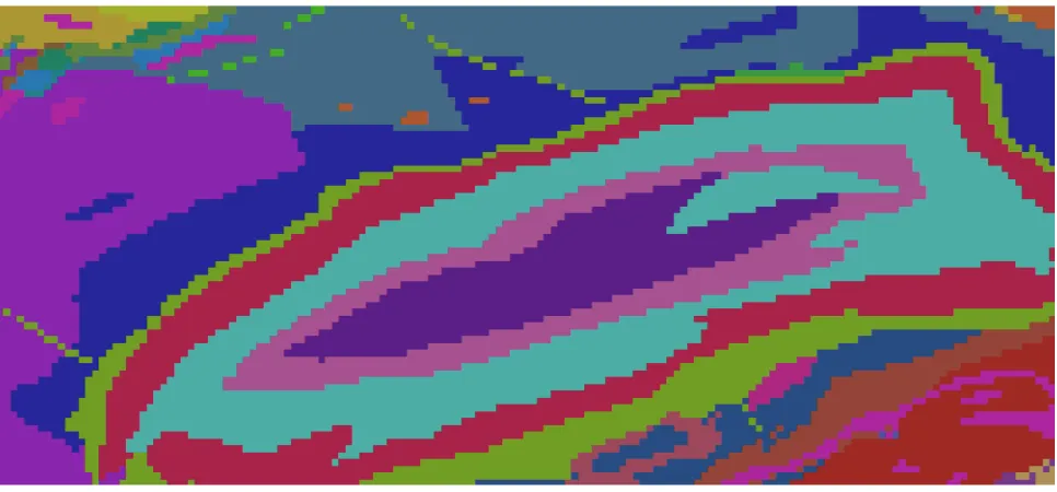
ratios were also used as feature inputs for calibration datasets and are summarized in Table 2. All the inputs features (i.e. total magnetic intensity, elevation, gravity, spectral images) are used to create a digital signature for each rocktype using calibration data, and used to identify unlabeled points during the classification. Rocktypes used to provide labels for calibration, classification, and validation datasets were provided by the Ontario Geological Survey (OGS) and can be seen in Figure 2 along with the descriptions and legend in Table 3 (Ontario Geological Survey, 2011).
Band Ratio Justification
3/1 Discriminating areas containing ferric iron associated with clays and alteration (Amen and Blaszczynski, 2001) 3/2 Discriminating areas containing carbonate rocks associated with clays and alteration (Durning et al., 1998) 3/5 Distinguish between calcareous sediment and mafic igneous rocks (Boettinger et al., 2008; Mshiu, 2011) 3/7 Identifying ferrous iron (Amen and Blaszczynkski, 2001)
5/1 Distinguish between volcanic and metamorphic rocks from sedimentary (Kusky and Ramadan, 2002) 5/2 Distinguish between calcareous sediment and mafic igneous rocks (Boettinger et al., 2008; Mshiu, 2011) 5/4 Identifying ferrous iron (Durning et al., 1998)
5/7 Discriminating areas containing hydroxyl ions associated with clays and alteration (Inzana et al., 2003) 5/4 * 3/4 Distinguish between volcanic and metamorphic rocks from sedimentary (Kusky and Ramadan, 2002)
Table 2. Landsat 4-5 TM band ratios that are used as input features for the calibration and classification datasets. Justification for each ratio is included. Adapted from Cracknell and Reading (2014).
Legend % Cover Rocktype Description
0.11 Amphibolite, gabbro, diorite, mafic gneisses
0.24 Basaltic and andesitic flows, tuffs and breccias, chert, iron formation, minor metasedimentary and intrusive rocks
7.07 Carbonaceous slate
0.08 Commonly layered biotite gneisses and migmatites; locally includes quartzofeldspathic gneisses, ortho- and paragneisses 0.44 Conglomerate, sandstone, siltstone, argillite
0.22 diorite, quartz diorite, minor tonalite, monzonite, granodiorite, syenite and hypabyssal equivalents 0.25 Gabbro, anorthosite, ultramafic rocks
0.82 Granite, alkali granite, granodiorite, quartz feldspar porphyry; minor related volcanic rocks (1.5 to 1.6 Ga)
13.54 Granophyre
18.53 Lapilli tuff, breccia, felsic flows and intrusions, minor carbonate and cherty
2.72 Mafic, intermediate and felsic metavolcanic rocks, intercalated metasedimentary rocks and epiclastic rocks 10.80 Massive to foliated granodiorite to granite
0.33 Murray Granite 2388 Ma, Creighton Granite 2333 Ma: granite
1.64 Nipissing mafic sills (2219 Ma): mafic sills, mafic dikes and related granophyre
0.14 Norite, gabbro, granophyre
7.79 Norite-gabbro, quartz norite, sublayer and offset rocks 0.24 Quartz sandstone, minor conglomerate, siltstone 3.50 Quartz-feldspar sandstone, argillite and conglomerate
0.38 Quartz-feldspare sandstone, sandstone with minor siltstone, calcareous siltstone and conglomerate
0.85 Rhyolitic, rhyodacitic, dacitic and andesitic flows, tuffs and breccias, chert iron formation, minor metaseds and intrusive rocks 0.09 Sandstone, siltstone, conglomerate, limestone, dolostone
0.13 Siltstone, argillite, sandstone, conglomerate 0.05 Siltstone, argillite, wacke, minor sandstone 2.33 Siltstone, wacke, argillite
10.70 Tonalite to granodiorite-foliated to gneissic-with minor supracrustal inclusions 10.40 Tonalite to granodiorite-foliated to massive
6.67 Wacke, minor siltstone
Table 3. Legend and rock type descriptions for Figure 2. Includes % of how much of the study area each rock type covers. Adapted from Ontario Geological Survey (2011).
3.2 Model Calibration
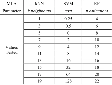
The optimal parameters specific to each of the 4 MLAs tested were determined through a 10-fold cross validation performed on calibration datasets composed of various cluster sizes and spatial distributions. The parameter values tested can be seen in Table 4. The optimal parameters were used as inputs for the prediction evaluation component of this study. The calibration data was composed of clusters, which was consistent at 20% of the study area data points. Each MLA was run for 2a clusters, where a = 0
to 9. This process was carried out over three trials for each MLA to account for the simple random seeding of clusters. This process can result in substantially different compositions of calibration points as a result of the seed locations and unequal quantities and non-uniform spatial distribution of each rocktype. The results of the cross validation for each trial were averaged for the final results of the model calibration. In both the calibration and final prediction evaluation components, simple random sampling in this study is assumed to be more representative of typical geological field mapping traverses and procedures than stratified sampling (Congalton, 1991).
MLA kNN SVM RF
Parameter k neighbours cost n estimators
Values
Table 4. Parameter and values tested for each MLA during the cross validation. The cross validation serves to determine which
3.3 Prediction Evaluation
The results for each MLA were assessed through (1) visualization of each classification, (2) classification juxtaposed with visualizations of correctly and incorrectly identified data points and cluster locations, and (3) overall performance assessment by percentage of correctly identified pixels. The purpose was to determine which MLA and under what conditions performs the best.
4. RESULTS
4.1 Cross Validation Results
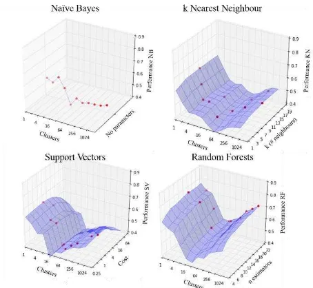
Figure 3 shows the results of the cross validation performed to determined optimal parameters to use in the prediction evaluation component of the study. The red dots in the figure show the best performance for each number of clusters for each MLA. The cross validation accuracies of all the MLAs show similar trends among each other as the number of clusters change, showing slightly better performance at the extremes of clusters and a trough centred around 16 to 64 clusters. Table 5 summarizes the performance for the best performing parameters for each MLA and corresponding clusters. Performance refers to percent of correctly identified pixels. The performance is poor, with best performance at 76%. This may be the result of a few factors. One large factor is likely the amount of vegetation coverage which hinders rock classification (see Cracknell and Reading, 2014 for geological mapping in a more suitable environment). Another factor here is that water bodies are not accounted for.
Figure 3. Comparison of the mean accuracies over three trials, i.e. varied calibration cluster locations, of the cross validation
for each MLA as functions of the number of clusters and parameter values to be tested as specified in Table 4. Red dots indicate best performance and parameter value that resulted in
the values used in the prediction evaluation, which are summarized in Table 5.
# Clusters Naïve Bayes k Nearest Neighbour Support Vector Machines Random Forest Performance k(neighbours) Performance Cost Performance n-Estimators Performance
1 54% 11 64% 4 65% 16 76%
2 51% 9 56% 8 61% 22 72%
4 57% 7 48% 2 55% 16 70%
8 49% 7 48% 2 54% 20 61%
16 37% 11 47% 2 37% 16 52%
32 43% 5 42% 1 42% 22 50%
64 41% 9 42% 0.5 43% 20 54%
128 42% 15 43% 0.5 47% 22 56%
256 42% 9 48% 0.5 51% 22 63%
512 43% 17 50% 2 52% 22 66%
Table 5. Accuracies for best performing parameter for each MLA and number of clusters from the cross validation. Best performance among clusters with corresponding parameter value for each MLA is highlighted in red.
4.2 Study Area Prediction Evaluation Results
Figure 4 shows the predictions and spatial distributions of correctly identified data points of the prediction evaluation
Figure 4. Visualizations of rocktype predictions, cluster distributions, and correctly identified data points for each MLA. Clusters = 1 and 512 are shown. The coloured image shows rocktype predictions with calibration pixels in lighter legend colours. Adjacent are
performance visualization images, where calibration pixels (light legend colours), correctly identified cells (grey) and incorrectly identified cells (black) can be seen. Refer to Figure 2 for the full rocktype map and Table 3 for the legend.
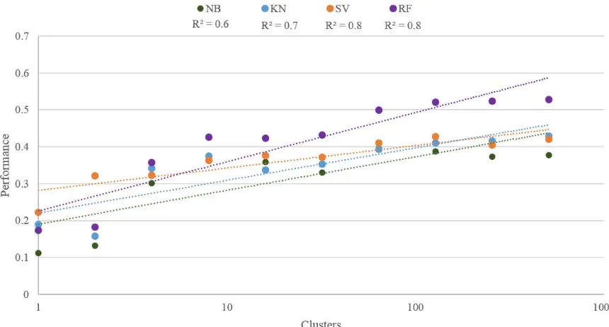
Figure 5 summarizes the overall performance of each classification, showing that performance for each MLA generally increases as the number of calibration clusters increases. Lin-log plot regression trend lines are included, as well as R2 values for each MLA. Naïve Bayes shows the poorest performance
generally. Naïve Bayes and k-nearest neighbour performed similarly with regards to the relationship between performance and number of clusters, however naïve Bayes fits the data the poorest of the four MLAs. Random forest overall produced the best results, steepest trend line, and best fitting data.
5. DISCUSSION
Generally results indicate that this is not a reliable technique for mapping lithology in regions that are heavily vegetated and have water coverage. Possibilities to mitigate these factors are to apply this technique in areas that have low vegetation, or weight inputs that rely on spectral response to be reduced. Another possibility is to group units that are similar in composition. This study considered rocktypes provided from the source material directly, however some units could reasonably be grouped together for this application. Rocktypes with similar composition and digital signatures may have been confused with one another resulting in reduced performance.
Increasing the number of clusters for calibration actualizes as an increased distribution of calibration points across the study area. A more uniform spatial distribution of calibration clusters increases the likelihood that all rocktypes are included in the calibration phase of the classification procedure. Additionally, this is more representative of non-preferential sampling, which can reduced biased inferences in interpretation (Diggle et al., 2010).
During the 10-fold cross validation, extremes for number of clusters (i.e. low and high) tested showed slightly better results. A low number of clusters could result in better performance in this case as the calibration points area all located in the same region spatially. These data are spatially constrained to an area that could reasonably have similar properties across it. A large calibration cluster could results in enough data within the same area to establish a distinct digital signature during the calibration phase of classification due to wide covered in a spatially constrained location. The trough in performance during the cross validation may be from the calibration clusters moving away from these spatially constrained area to being less spatially defined. However, as number of clusters increases to 512, there is wider spatial coverage across the entire study area, presenting a circumstance once again where a wide portion of the study area is covered and spatial coordinates are valuable as feature inputs for classification.
During the prediction evaluation across the entire study area, MLA predictions improve as the number of clusters increase (lin-log scale). This follows similar (lin-logic to the improving performance for the higher number of clusters during the cross validation, however fewer calibration clusters for the entire dataset results in poorer performance, which differs from the cross validation. In the cross validation, only the rocktypes in the calibration data region were considered. Fewer clusters for the entire study area result in limited, and sometimes zero, access to each rocktype. If a labelled rocktype is not available during the calibration phase, the MLA will not be able to assign the correct class label during the classification phase. The assertion that performance improves with a greater number of clusters can be observed in the prediction and error location maps (Figure 4). The performances are best summarized by the overall accuracy, Figure 5, which shows naïve Bayes as the poorest performing MLA and random forest as the best. Random forest here shows the most promise in this application, however it can be subject to
6. CONCLUSIONS
The use of other geophysical data, specifically total magnetic intensity, digital elevation, and Bouguer gravity anomaly, as input classification features was found to be useful for “first-pass” assessments and interpretation of geological rocktypes. Typically, prior to a field visit, a geologist will recover all known geological information about a site. This allows for delineating regions of interest and structural trends that may exist in the area. This includes possible contacts among rock units, which are often hidden under surface material (e.g. vegetation, soil) and inferred through interpretations from outcrop to outcrop. A geologist in the field will map rock outcroppings and must know what to look for, including structural and contact trends. The assertions of this study support previous studies that random forest is the best performing MLA for this application. However, it was found that due to the considerably low performance of even the best MLA, this approach cannot be used to replace proper site investigation for geological mapping and ground validation. It can however, be used at the desktop study (phase I site investigation) state in order to plan effective field traverses that could enhance geological interpretations.
REFERENCES
Amen, A. & Blaszczynski, J., 2001. Integrated Landscape Analysis. U.S. Department of the Interior, Bureau of Land Management, National Science and Technology Center, Denver, CO, USA, pp. 2-20.
Boettinger, J.L., Ramsey, R.D., Bodily, J.M., Cole, N.J., Kienast-Brown, S., Nield, S.J., Saunders, A.M., & Stum, A.K., 2008. Landsat Spectral Data for Digital Soil Mapping. In: Hartemink, A.E., McBratney, A. B. and Mendonça -Santos, M. de L. (Ed.), Digital Soil Mapping with Limited Data. Springer, Netherlands, pp. 192-202.
Bond, C.E., Gibbs, A.D., Shipton, Z.K., & Jones, S., 2007. What do you think this is? “Conceptual uncertainty”. In: Geoscience Interpretation. GSA Today, 17(11), pp. 4-10.
Breiman, L., (2001). Random forests. Machine Learning. pp. 5-32.
Congalton, R.G., 1991. A review of assessing the accuracy of classifications of remotely sensed data. Remote Sensing of Environment, 37(October 1990), pp. 35-46.
Cortes, C., & Vapnik, V., 1995. Support-vector networks. Machine Learning, 20, pp. 273-297.
Cracknell, M.J., & Reading, A.M., 2014. Geological mapping using remote sensing data: A comparison of five machine learning algorithms, their response to variations in the spatial distribution of training data and the use of explicit spatial information. Computers & Geosciences, 63, pp. 22-33.
mineralisation using spectral sensing techniques at Woodie Woodie, East Pilbara. Exploration Geophysics, 37(4), pp. 389-400.
Inzana, J., Kusky, T., Higgs, G., & Tucker, R., 2003. Supervised classifications of Landsat TM band ratio images and Landsat TM band ratio image with radar for geological interpretations of central Madagascar. J. Afr. Earth Sci. 37, pp. 59-72.
Kusky, T.M. & Ramadan, T.M., 2002. Structural controls on Neoproterozoic mineralization in the South Eastern Desert, Egypt: an integrated field, Landsat TM, and SIR-C/X SAR approach. J. Afr. Earth Sci. 35, pp. 107-121.
Massironi, M., Bertoldi, L., Calafa, P., Visonà, D., Bistacchi, A., Giardino, C., & Schiavo, A., 2008. Interpretation and processing of ASTER data for geological mapping and granitoids detection in the Saghro massif (eastern Anti-Atlas, Morocco). Geosphere, 4(4), pp. 736-759.
Mshiu, E.E., 2011. Landsat remote sensing data as an alternative approach for geological mapping in Tanzania: a case study in the Rungwe Volcanic Province, south-western Tanzania. J. of Sci. 37, pp. 26-36.
Munyati, C., 2000. Wetland change detection on the Kafue Flats, Zambia, by classification of a multitemporal remote sensing image dataset. International Journal of Remote Sensing, 21(9), pp. 1787-1806.
Ontario Geological Survey, 2011. 1:250 000 scale bedrock geology of Ontario. Ontario Geological Survey, Miscellaneous Release - Data 126 - Revision 1.
Ontario Geological Survey, 2011. Single master gravity and aeromagnetic data for Ontario. Ontario Geological Survey Ministry of Northern Development and Mines, 1035.
Pedregosa, F., & Varoquaux, G., 2011. Scikit-learn: Machine learning in Python. Journal of Machine Learning Research, 12, pp. 2825-2830.
Peredery, W.V., 1991. The Geology and Ore deposits of the Sudbury Structure, Ontario. Ontario Geological Survey.
Rowan, L.C., & Mars, J.C., 2003. Lithologic mapping in the Mountain Pass, California area using Advanced Spaceborne Thermal Emission and Reflection Radiometer (ASTER) data. Remote Sensing of Environment, 84, pp. 350-366.
Sabins, F. F., 1999. Remote sensing for mineral exploration. Ore Geology Reviews, 14, pp. 157-183.
United States Geological Survey, 2011. Landsat 4-5 Imagery, October 2011. Retrieved March 2014.
United States Geological Survey, 2000. Shuttle Radar Topography Mission 1 Arc-Second Global Elevation Data. Retrieved March 2014.