Universal Low Temperature Asymptotics of
the Correlation Functions of the Heisenberg Chain
⋆Nicolas CRAMP ´E †, Frank G ¨OHMANN ‡ and Andreas KL ¨UMPER ‡
† LPTA, UMR 5207 CNRS-UM2, Place Eug`ene Bataillon, 34095 Montpellier Cedex 5, France
E-mail: [email protected]
‡ Fachbereich C – Physik, Bergische Universit¨at Wuppertal, 42097 Wuppertal, Germany
E-mail: [email protected],[email protected]
Received August 18, 2010, in final form October 04, 2010; Published online October 09, 2010
doi:10.3842/SIGMA.2010.082
Abstract. We calculate the low temperature asymptotics of a function γ that generates the temperature dependence of all static correlation functions of the isotropic Heisenberg chain.
Key words: correlation functions; quantum spin chains; thermodynamic Bethe ansatz
2010 Mathematics Subject Classification: 81Q80; 82B23
1
Introduction
Over the past few years the mathematical structure of the static correlation functions of the XXZ chain was largely resolved. After an appropriate regularization by a disorder parameter they all factorize into polynomials in only two functions ρ and ω [8]. These are the one-point function and a special neighbor two-point function which, in turn, can be represented as integrals over solutions of certain linear and non-linear integral equations [2]. This resembles much the situation with free fermions, and what is behind is indeed a remarkable fermionic structure on the space of quasi-local operators acting on the spin chain [5]. It allows us, for instance, to calculate short-range correlators with high numerical precision directly in the thermodynamic limit [1,12].
The low temperature asymptotics of ρ and ω universally determines the low temperature properties of all static correlation functions. In this short note we obtain the low temperature asymptotics in the special case of the isotropic Hamiltonian
H=JX
j
σxj−1σxj +σyj−1σyj +σj−z 1σjz (1.1)
with no magnetic field applied and vanishing disorder parameter. Then ρ = 1 and we are left with only one function (and its derivatives) which, up to a trivial factor, is the functionγ defined in [3].
2
Def inition of the basic function
γ
For our purpose here it is convenient to introduce the function γ within the context of a special realization of a six-vertex model (see e.g. [4]) and its associated quantum transfer matrix [10].
By definition the latter has 2(N+M) vertical lines alternating in direction and carrying spectral
The spectral parameter on the horizontal line will be denoted µ2. We consider this system in the limit N,M → +∞ with the fine tuning uN = iJT and u′M= iTδ. With an appropriate overall normalization the largest eigenvalue Λ(µ2, µ1) is given by
ln(Λ(µ2, µ1)) =
Let us note that we recover the familiar system of equations, allowing us to study the thermo-dynamical properties of the Hamiltonian (1.1), by setting δ = 0. The functionK(x) is defined as
where ψ is the digamma function. The auxiliary functionsb(x, µ) and b(x, µ) are solutions of a pair of non-linear integral equations given by
ln(b(x, µ1)) =− 2πJ
It has been conjectured [3] that the correlation functions of the isotropic Heisenberg chain at any finite temperature (for vanishing magnetic field) are polynomials in γ and its derivatives evaluated at (0,0). A similar statement (involving a function ω and its derivative with respect to the disorder parameter) was proved for the anisotropic XXZ chain [5,8,2]. Amazingly the isotropic limit seems non-trivial and is still a subject of ongoing work. Here we would only like to mention that the nearest- and next-to-nearest-neighbor two-point functions were expressed in terms of γ in [3] starting from the multiple integral representation for the density matrix of the Heisenberg chain obtained in [7]. The formulae for the longitudinal two-point functions are, for instance,
3
Low-temperature expansion
To compute the low-temperature expansion ofγ, we follow the line of reasoning of the article [9], where a similar task was performed for the free energy. There are, however, two differences between the usual equations and the ones used in this note: the additional driving term in (2.2) proportional toδ and the shift µ2 in the kernel of the integration in (2.1).
The computation is based on the introduction of a shift L = π1ln πJT in the auxiliary functions:
bL(x) =b(x+L) and ebL(x) =b(−x− L).
In the low-temperature limit these functions satisfy
ln(bL(x, µ1))∼ −4e−πx−4δ
where DL(x) is the rest of the integral which does not contribute to the low-temperature limit,
when the magnetic field vanishes (see [9]). A similar relation holds with b ↔ b and i ↔ −i exchanged.
In terms of the shifted functions the largest eigenvalue becomes
ln(Λ(µ2, µ1))∼ 4πJ
To evaluate these integrals we compute
I =
Z ∞
−L
dtln(1 +bL(t, µ1)) ln(bL(t, µ1))′+ ln(1 +bL(t, µ1)) ln(bL(t, µ1))′
using two different methods. Here the prime stands for the derivative with respect to t. First, we compute it explicitly using the change of variables z = ln(bL) or z = ln(bL), respectively, which results in resulting expression by taking into account that the derivative ofK(x) is odd and contributions by double integrals cancel pairwise. This way we obtain
I = 4π
The same type of manipulation can be performed for the functions eb, and a similar result is obtained with µ1 replaced by −µ1.
Gathering these findings we obtain the asymptotic form of the largest eigenvalue,
0 0.05 0.1 0.15 0.2 0.25
1e-02 1e-01 1e+00 1e+01 1e+02
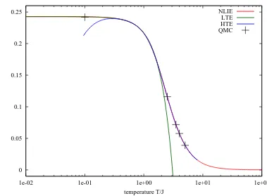
next-to-nearest neighbour zz-correlation function
temperature T/J
NLIE LTE HTE QMC
Figure 1. Comparison of the high- and low-temperature expansions (HTE, LTE) of hσz 1σ
z
3i with the
full numerical solution obtained from the integral equations (NLIE) and with Monte-Carlo data (QMC).
Thus, using (2.3), the function γ behaves asymptotically for small temperatures as
γ(µ1, µ2)∼ −1 + 1 + (µ1−µ2)2
4πK(µ2−µ1)− T2
12J2cosh(π(µ1+µ2))
.
This is our main result.
Using (2.4) and (2.5), we obtain the low-temperature expansion of the longitudinal correlation functions
hσz1σ2ziT ∼
1 3−
4
3ln(2) + T2 J2
1 36,
hσz1σ3ziT ∼
1 3−
16
3 ln(2) + 3ζ(3)− T2 J2
1 36
π2 2 −4
.
The constant terms (independent of the temperature) in these expansions are in agreement with those originally found in [11, 6]. In the figure we compare the combined low- and high-temperature results for the next-to-nearest neighbor zz-correlation functions with the full nu-merical curve obtained by implementing the linear and non-linear integral equations that deter-mine γ and its derivatives [3] on a computer. The high-temperature data and some additional Monte-Carlo data are taken from [14]. We find that the numerical curves (NLIE, QMC) are amazingly well approximated by its low- and high-temperature approximations.
Acknowledgments
References
[1] Boos H., Damerau J., G¨ohmann F., Kl¨umper A., Suzuki J., Weiße A., Short-distance thermal correlations in the XXZ chain,J. Stat. Mech. Theory Exp.2008(2008), P08010, 23 pages,arXiv:0806.3953.
[2] Boos H., G¨ohmann F., On the physical part of the factorized correlation functions of the XXZ chain,
J. Phys. A: Math. Theor.42(2009), 315001, 27 pages,arXiv:0903.5043.
[3] Boos H., G¨ohmann F., Kl¨umper A., Suzuki J., Factorization of multiple integrals representing the density matrix of a finite segment of the Heisenberg spin chain,J. Stat. Mech. Theory Exp.2006(2006), P04001,
13 pages,hep-th/0603064.
[4] Boos H., G¨ohmann F., Kl¨umper A., Suzuki J., Factorization of the finite temperature correlation functions of theXXZ chain in a magnetic field,J. Phys. A: Math. Theor.40(2007), 10699–10728,arXiv:0705.2716.
[5] Boos H., Jimbo M., Miwa T., Smirnov F., Takeyama Y., Hidden Grassmann structure in theXXZ model. II. Creation operators,Comm. Math. Phys.286(2009), 875–932,arXiv:0801.1176.
[6] Boos H.E., Korepin V.E., Quantum spin chains and Riemann zeta function with odd arguments,J. Phys. A: Math. Gen.34(2001), 5311–5316,hep-th/0104008.
[7] G¨ohmann F., Kl¨umper A., Seel A., Integral representation of the density matrix of theXXZchain at finite temperature,J. Phys. A: Math. Gen.38(2005), 1833–1841,cond-mat/0412062.
[8] Jimbo M., Miwa T., Smirnov F., Hidden Grassmann structure in the XXZ model. III. Introducing Matsubara direction,J. Phys. A: Math. Theor.42(2009), 304018, 31 pages,arXiv:0811.0439.
[9] Kl¨umper A., The spin-1/2 Heisenberg chain: thermodynamics, quantum criticality and spin-Peierls expo-nents,Eur. Phys. J. B5(1998), 677–685,cond-mat/9803225.
[10] Suzuki M., Transfer-matrix method and Monte-Carlo simulation in quantum spin systems,Phys. Rev. B31
(1985), 2957–2965.
[11] Takahashi M., Half-filled Hubbard model at low temperature,J. Phys. C10(1977), 1289–1301.
[12] Trippe C., G¨ohmann F., Kl¨umper A., Short-distance thermal correlations in the massiveXXZ chain,Eur. Phys. J. B73(2010), 253–264,arXiv:0908.2232.
[13] Tsuboi Z., A note on the high temperature expansion of the density matrix for the isotropic Heisenberg chain,Phys. A377(2007), 95–101,cond-mat/0611454.