El e c t ro n ic
Jo ur
n a l o
f P
r o
b a b il i t y
Vol. 15 (2010), Paper no. 5, pages 110–141. Journal URL
http://www.math.washington.edu/~ejpecp/
Expected Lengths of Minimum Spanning Trees for
Non-identical Edge Distributions
Wenbo V. Li
∗Department of Mathematical Sciences University of Delaware
Newark, DE, 19716 Email: [email protected]
Xinyi Zhang
†Division of Public Health Sciences Fred Hutchinson Cancer Research Center
Seattle, WA, 98109 Email: [email protected]
Abstract
An exact general formula for the expected length of the minimal spanning tree (MST) of a connected (possibly with loops and multiple edges) graph whose edges are assigned lengths according to independent (not necessarily identical) distributed random variables is developed in terms of the multivariate Tutte polynomial (alias Potts model). Our work was inspired by Steele’s formula based on two-variable Tutte polynomial under the model of uniformly identi-cally distributed edge lengths. Applications to wheel graphs and cylinder graphs are given under two types of edge distributions.
Key words:Expected Length, Minimum Spanning Tree, The Tutte Polynomial, The Multivariate Tutte Polynomial, Random Graph, Wheel Graph, Cylinder Graph.
AMS 2000 Subject Classification:Primary 60C05; Secondary: 05C05, 05C31. Submitted to EJP on January 5, 2009, final version accepted January 15, 2010.
∗Supported in part by NSF Grant No. DMS-0505805
1
Introduction
For a finite and connected graphG = (V,E) with vertex set V and edge set E, we denote the total length of its minimum spanning tree (MST) as
LM S T(G) = X
e∈E(M S T(G))
ξe, (1)
where ξe is the length of the edge e ∈ E. We are interested in studying the expected length of the MST of G, denoted asELM S T(G), for nonnegative random variablesξe with independent (not necessarily identical) distribution Fe. For the special case that Fe = F for every edge e, we use notationELF
M S T(G). In particular, ifF is the uniform distribution on the interval(0, 1), i.e.,U(0, 1), or exponential distribution with rate 1, i.e., exp(1), then the expected length of the MST of the graphG is denoted asELu
M S T(G)orELeM S T(G)respectively. Frieze[Fri85]first studiedELF
M S T(G)and showed that for a complete graphKn onnvertices,
lim n→∞EL
F
M S T(Kn) =ζ(3)/F′(0), wher eζ(3) = ∞ X
k=1
k−3=1.202....
This implies that
lim n→∞EL
e
M S T(Kn) =nlim→∞ELuM S T(Kn) =ζ(3).
Later, this result was extended and strengthened in many different ways, refer to [Ste87; FM89; Jan95]. Moreover, Steele [Ste02] started the investigation on exact formulae for the expected lengths of MSTs and discovered the following nice formula
ELu
M S T(G) = Z 1
0
(1−t) t
Tx(G; 1/t, 1/(1−t))
T(G; 1/t, 1/(1−t)) dt, (2)
where T(G;x,y) is the standard Tutte polynomial of G and Tx(G;x,y) is the partial derivative of T(G;x,y) with respect to x. This can be easily extended, see [LZ09], to the case of general independent and identical distributed (i.i.d.) edge lengths as
ELF
M S T(G) = Z ∞
0
1−F(t)
F(t)
Tx(G;x,y)
T(G;x,y) dt, (3)
where x =1/F(t), y =1/(1−F(t)). For discussions about the standard Tutte polynomial and the multivariate Tutte polynomial, see Section 2.
In this paper, we provide an exact formula for the expected lengths of MSTs for any finite, connected graphG, in which the edge length distributions are not necessarily identical. This generalizes for-mulae (2) and (3) considerably.
Theorem 1 (General Formula). Let G = (V,E) be a finite, connected graph, in which each edge e ∈ E has a positive random length ξe with independent distribution Fe(t) = P(ξe ≤ t). If we set
E′(t) ={e: 0<Fe(t)<1}and G′(t) =G/{e:Fe(t) =1}, then
ELM S T(G) =
Z ∞ 0
Y
e∈E′(t) 1 1+ve(t)
Zq(G′(t); 1,v(t))−1
dt, (4)
where ve(t) =Fe(t)/(1−Fe(t)),v(t) ={ve(t),e∈E′(t)}, and Zq(G′(t); 1,v(t))is the partial deriva-tive of the multivariate Tutte polynomial Z(G′(t);q,v(t))with respect to q evaluated at q=1.
Note that if the edge length distributions are i.i.d., then the above formula is reduced to (3) by relations between the multivariate Tutte polynomial and the standard Tutte polynomial. See Section 2 for more details.
The seemingly complicated general formula applied to specific graphs shows a more explicit form. In this paper, the applications of this generalized formula are illustrated in two families of graphs: wheel graphs and cylinder graphs. These graphs are assumed to have two different types of edges following two different types of edge length distributions. In particular, we are interested inU(0, 1)
and exp(1)edge length distributions. By applying our generalized formula, we compareELM S T(G)
between graphs with switched edge types. In addition, we show that Theorem 1 also provides a new angle to work on the problem of the expected lengths of MSTs of the complete graph. For more applications of Theorem 1, refer to[Zha08].
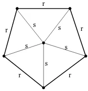
A wheel graph, see Figure 1 for an example, is often used in network to illustrate the simple topology. To distinguish the two different type of edges, we use dark and thick lines to draw rims, and lighter and thinner lines to draw spokes. The lettersr andsbeside the edges indicate the edge type as rim and a spoke respectively.
Definition 1 (Wheel Graphs with two types of edges). The wheel graph Wn is defined as the joint
K1+Cn, where K1is the (trivial) complete graph on 1 node (which is known as the hub) and Cn is the cycle graph of n vertices. The edges of Cnare calledrimsand the edges of a wheel which include the hub are calledspokes.
r
r
r
r r
s
s s
s
s
Figure 1: Wheel GraphW5 with Two Types of Edges
Theorem 2. For a wheel graph Wn with the nonnegative lengths of rims and spokes following dis-tributions Fr(t) = P(ξr ≤ t) and Fs(t) = P(ξs ≤ t) respectively, if we assume b = min{t :
(Fr(t)−1)(Fs(t)−1) =0}, then
lim n→∞
1
nELM S T(Wn) =
Z b
0
(1−Fr(t))2(1−Fs(t))
1−Fr(t) +Fr(t)Fs(t) dt.
Note that b in the above theorem is allowed to be infinity, see discussions in Section 4.1.2. The-orem 2 shows that ELM S T(Wn) converges to a constant with a scaling of the number of vertices.
Comparing the expected length of the wheel graph with that of the complete graph, the cubic graph [Pen98]and the almost regular graph studied in[BFM98; FRT00], we see that the scaling of con-vergence is related to the graph density. Recall that for a simple graphG= (V,E), the graph density is defined as
D(G) = 2|E|
|V|(|V| −1).
One may check that all the graphs mentioned above satisfy the following identity:
lim
n→∞D(G)EL u
M S T(G) =CG,
for some constantCG. We conjecture that this identity holds for all simple graphs.
If we specify the two types of edge length distribution in the wheel graph as U(0, 1) and exp(1), then the asymptotic values ofELM S T(Wn)/nfollow immediately after Theorem 2. In addition, we
compare ELue
M S T(Wn)/nand ELeuM S T(Wn)/n, the values of the expected length of the MST for the wheel graph with switched edge length distributions. See Section 4.1 for more details.
As another example, we apply Theorem 1 to the cylinder graph Pn×Ck, which was studied by Hutson and Lewis[HL07]under i.i.d uniform distribution. Since it is natural to divide the edges of the cylinder graph into two types, we study ELM S T(Pn×Ck) under general non-identical edge distribution.
Definition 2 (Cylinder Graphs with two types of edges). A cylinder graph of length n is defined as
Pn×Ck, a Cartesian product of a path Pn and a cycle Ck. The edges on the paths Pnand the cycles Ck are called type 1 edges and type 2 edges respectively.
1
1
2 1
2 1
2
1
1
2
2 2
2 2
2 2
2 2
1 1
Figure 2: The CylinderP2×C4 with Two types of Edges
Following similar ideas in [HL07], but with more complicated derivation and identifying various quantities, we obtain a representation of Z(Pn×Ck) in terms of Z(P0×Ck)and a transfer matrix
Theorem 3. For a cylinder graph Pn×Ckwith k≥2, letλ(q,v)be the Perron-Frobenius eigenvalue of the transfer matrix A(q,v), defined in (25).
(a). If the edges on the paths and cycles have lengths following distributionsexp(1)and U(0, 1) respec-tively, then
lim n→∞
1
nEL
eu
M S T(Pn×Ck) =
e−k
k +
Z 1
0
λq(1,v(t))
λ(1,v(t)) dt, wherev(t) ={v1(t),v2(t)}, v1(t) =et−1and v2(t) =t/(1−t).
(b). If the edges on the paths and cycles have lengths following distributions U(0, 1)andexp(1) respec-tively, then
lim n→∞
1
nEL
ue
M S T(Pn×Ck) = Z 1
0
λq(1,u(t))
λ(1,u(t)) dt, whereu(t) ={u1(t),u2(t)}, u1(t) =t/(1−t)and u2(t) =et−1.
Note that the two integrals in cases (a) and (b) are different. From numerical results in Table 3, we conjecture that the integral in (a) is bigger than the one in (b). Thus, if normalized by the length of the cylinder graph, we conjecture that the asymptotic value ofELeu
M S T(Pn×Ck)is always bigger thanELue
M S T(Pn×Ck)by a quantity larger thane−k/k.
Our proposed general formula also applies to non-simple graphs, i.e. graphs with loops (edges join-ing a vertex to itself) or multiple edges (two or more edges connectjoin-ing the same pair of vertices). This feature together with the non-i.i.d. edge length assumption enables us to study the random minimum spanning tree problem in much more complicated situations. In addition, this general-ized formula applied to the complete graph serves as a general formula for the expected length of any simple connected graph. The remaining of the paper is organized as follows: We discuss the main properties of the multivariate Tutte polynomial related to our results and compare it with the standard Tutte polynomial in Section 2. These are also used in the proof of Theorem 1 in Section 3, where the relationship between the standard Tutte polynomial and the expected length of MST is reviewed and analyzed. In Section 4, several applications of Theorem 1 are given.
2
The Multivariate Tutte Polynomial
The multivariate Tutte polynomial has been known to physicists for many years in various forms, but it is relative new to mathematicians. The first comprehensive survey was given by Sokal[Sok05]. Since the multivariate Tutte polynomial contains all the edge lengths as variables, it is generally considered to be more flexible to use than its two-variate version (standard Tutte polynomial). For example, it allows simpler forms of deletion-contraction identity and parallel-reduction identity. In this section, we first review basic properties of the multivariate Tutte polynomial and compare it with the standard Tutte polynomial. Then the relationship of the general formula (4) with formulae (2) and (3) is explored, Finally, we discuss how the application of this formula to the complete graph generalizes the expected lengths of MSTs of all finite simple graphs.
Definition 3(The Standard Tutte polynomial). The Tutte polynomial of a graph G is a two-variable
polynomial defined as
T(G;x,y) =X
A⊆E
where k(A) denotes the number of connected components in the subgraph(V,A), and r(A) is the rank function defined as r(A) =|V| −k(A).
The standard Tutte polynomial is a special case of the multivariate Tutte polynomial.
Definition 4 (The Multivariate Tutte Polynomial). For a finite graph G = (V,E) (not necessarily
simple or connected), its multivariate Tutte polynomial is defined as
Z(G; q, v) =X
A⊆E
qk(A)Y
e∈A
ve, (6)
where q andv={ve, e∈E}are variables.
If we set the edge weights ve to the same value v, then a two-variable polynomial Z(G;q,v) is obtained, which is essentially equivalent to the standard Tutte polynomialT(G;x,y)in the following way:
T(G;x,y) = (x−1)−k(E)(y−1)−|V|Z(G;(x−1)(y−1),y−1). (7) From Definition 4, we can see that by setting q = 1, the multivariate Tutte polynomial is much simplified as
Z(G; 1,v) =X
A⊆E Y
e∈A
ve=Y
e∈E
(1+ve). (8)
Actually as formula (7) shows,q=1 in Z(G;q,v)corresponds to(x−1)(y−1) =1 inT(G;x,y). Thus, by applying (7) and settingve=v= y−1 in (8), one easily obtains the well-known simplied version of the standard Tutte polynomial on the hyperbolaH1={(x−1)(y−1) =1}as
T(G;x,y) =x|E|(x−1)|V|−k(E)−|E|. (9) While it may not be that easy to observe that the standard Tutte polynomial simplifies on H1, the simplification ofZ(G;q,v)atq=1 is almost trivial to see.
In the practice of computing the multivariate Tutte polynomial for specific graphs, it is usually hard to apply Definition 4 directly. The following identities, which can be verified by Definition 4, for the multivariate Tutte polynomial are often used to simplify the computation. Moreover, these identities are usually in simpler forms than their two-variate versions. For a detailed discussion of the multivariate Tutte polynomial, we refer to[Sok05].
Union Graph Identity
1. If graphsG1 andG2are disjoint, then
Z(G1∪G2;q,v) =Z(G1;q,v)Z(G2;q,v).
2. If graphsG1 andG2share one common vertex but no common edges, then
Z(G1∪G2;q,v) =
Z(G1;q,v)Z(G2;q,v)
Duality Identity
For a connected planar graphG= (V,E), letG∗= (V∗,E∗)be its dual graph, then
Z(G;q,v) =q|V|−|E|−1 Y
e∈E
ve
!
Z G∗;q,q/v
. (11)
Deletion-Contraction Identity
For anye∈E,
Z(G;q,v) =Z(G\e;q,v6={e}) +veZ(G/e;q,v6={e}), (12) wherev6={e}={vf,f ∈E\e}. In particular, ifeis a loop or bridge, then this identity is simplified as
Z(G;q,v) =
¨
(1+ve)Z(G/e;q,v), ifeis a loop
(q+ve)Z(G/e;q,v), if eis a bridge .
Note that a bridge in a connected graph is defined as an edge whose removal disconnects the graph.
Parallel-Reduction Identity
Another useful feature of the multivariate Tutte polynomial is the simple parallel-reduction identity. That is, we can replacem parallel edgese1, . . . ,em, which join the same pair of vertices x,y, by a single edgeewith weight
ve= m Y
i=1
(1+vei)−1, (13)
without changing the value of the multivariate polynomial Z.
From Theorem 1, we see that if all the edge lengths follow an identical distribution F, thenve(t) = v(t) = F(t)/(1− F(t)) for any e ∈ E and Z(G;q,v(t)) becomes a two-variate polynomial. For
y=v(t) +1 and x=q/v(t) +1,
Z(G;q,v(t)) = (x−1)(y−1)|V|T(G;x,y), and
Zq(G;q,v) = (y−1)|V|−1T(G;x,y)
(x−1)Tx(G;x,y) T(G;x,y) +1
.
Specifically, forq= (x−1)(y−1) =1,T(G;x,y) =x|E|(x−1)|V|−|E|−1. Therefore,
Zq(G; 1,v) = y|E|
(x−1)Tx(G;x,y) T(G;x,y) +1
,
where(x−1)(y−1) =1. This shows that for i.i.d. edge lengths, the general formula (4) is reduced to formula (3). In addition, if the identical edge length distribution is specified to be U(0, 1), then by settingx =1/t and y =1/(1−t), one obtains Steele’s formula (2).
with large lengths to G. To be more precise, for any two vertices i, j ∈ V, if the edge i j ∈/ E, then setξi j = M and E=E∪i j. Eventually, a complete graphKn is formed. If the supplemented edge length M is chosen to be a large number, say M = max{ξe,e ∈ E}+1, then there is no chance for the supplemented edges to be selected in the MST. Therefore,ELM S T(G)is the same as
the expected length of MST for the complete graphKn, on which the edge weight ξ′e satisfies the following condition:
ξ′e=
¨
ξe, ife∈E,
M, ife∈/E.
Therefore, it is useful to exam the multivariate Tutte polynomial of a complete graph, more details are discussed in Section 4.3.
3
Proof of the Main Theorem
It is well known that the length of MST of a graph with random edge lengths can be represented in terms of the number of components, refer to[AB92; Ste02; Jan95]for edge lengths distributed uniformly on the interval(0, 1)and[Gam05; LZ09]for simple, finite, connected graphs with general i.i.d. nonnegative edge distributions. The essence of the idea is summarized in the following lemma. For the completeness, we include its proof. Note that this lemma is not restricted to simple graph or identical edge distributions. It holds for graphs with non-random edge lengths as well.
Lemma 1. For any finite, connected graph G= (V,E)(not necessarily simple) with independent
ran-dom edge lengths, we have
LM S T(G) =
Z ∞ 0
(k(t)−1)dt,
where k(t)is the number of components in the random graph G(t) = (V,E(t))where the edge set E(t) is defined to consist of all edges in G with length no more than t.
Proof:Given a finite, connected graphG= (V,E), consider a continuous time random graph process
G(t) = (V,E(t))with the edge setE(t) ={e:ξe≤t}. LetN(t)be the number of MST edges selected up to timet,i.e.,
N(t) = X
e∈E(t)
I(e∈E(M S T(G))) =
X
e∈E(M S T(G))
I(ξe≤t).
Thenk(t) =|V|−N(t), since the selection of each MST edge in the random graph process decreases the number of components by 1.
Hence a nice representation for the length of MST is obtained as the following:
LM S T(G) = X
e∈E(M S T(G))
ξe= X
e∈E(M S T(G))
Z ∞ 0
I(t< ξe)dt
=
Z ∞ 0
X
e∈E(M S T(G))
(1−I(ξe≤t))dt
=
Z ∞ 0
(|V| −1−N(t))dt=
Z ∞ 0
Note that the integration limit is only up to maxe∈E(G)ξe, sincek(t) =1 for t >maxe∈E(G)ξe, ifG
is connected. This finishes the proof of Lemma 1. One can check that the above argument does not requireGto be a simple graph, since neither a loop nor a multiple edge can be selected in the MST
ofG.
Proof of Theorem 1: Inspired by Steele’s work [Ste02], we relate k(t) to the multivariate Tutte
polynomial of the graphG(t). In this way, we not only allow the graph to have multiple edges and loops, but also allow the edge weights to follow non-identical distributions. Assume ξe ∼ Fe(t), then the moment generating function ofk(t)is
φ(s) =Eexp(sk(t)) =
X
A⊆E Y
e∈A
Fe(t)
!
Y
e∈E\A
(1−Fe(t))
e
sk(A).
Since the edge lengths may follow different distributions, it is possible that for some t > 0, there exists an edge esuch that Fe(t) =1. Let E′(t) ={e∈E: Fe(t)<1}, then φ(s)is the same as the above formula with the edge setEreplaced by E′(t).
Let G′(t) be the graph obtained from G(t) by contracting each pair of endpoints of the edge in
E\E′(t) into a single vertex (loops may be formed). Then we can rewrite φ(s) in terms of the multivariate Tutte polynomial as the following:
φ(s) = Y
e∈E′(t)
1−Fe(t)
X
A⊆E′(t)
esk(A) Y
e∈A
Fe(t)
1−Fe(t)
!
= Y
e∈E′(t) 1 1+ve(t)
Z(G′(t); es, v(t)),
wherev(t) ={ve(t), e∈E′(t)}andve(t) =Fe(t)/(1−Fe(t)).
Therefore, if we denoteZq(G;q,v)as the partial derivative of the multivariate Tutte polynomial with respect toq, then
Ek(t) =φ′(0) = Y
e∈E′(t) 1
1+ve(t) Zq(G
′(t); 1, v(t)).
This finishes the proof of Theorem 1.
4
Applications
Theorem 1 gives a most generalized version of the exact formula ofELM S T(G)in the sense that it not only allows the edge distributions to be non-identical, but also allows the graphs to be non-simple. In this section, we apply this general theorem to two specific families of graphs: wheel graphs and cylinder graphs. For both families of graphs, the edges are divided into two groups by the type of edge length distribution. We first derive the multivariate Tutte polynomial explicitly, then study the exact values and asymptotic values of the expected lengths of MSTs. At the end of this section, we apply Theorem 1 to complete graphs. Since Frieze[Fri85]first studied ELF
4.1
The Wheel Graph
The wheel graph, defined in Section 1, is an important class of planar graphs both in theory and in applications. It has nice properties such as self-duality, see[ST50; Tut50]. In[LZ09], the wheel graph was used as an example to study the expected length of MST for graphs with general i.i.d. edge lengths. In this paper, we consider the wheel graphs with rims and spokes following edge distributionsFr andFs respectively. The graph structure of the wheel graph enables us to compute its multivariate Tutte polynomial with two types of edges explicitly. By applying the general formula (4), we obtain a representation ofELM S T(Wn). In Section 4.1.2, we substituteU(0, 1) and exp(1) distributions as special cases ofFr andFs and compute the exact values and asymptotical values of the expected lengths of MSTs for the wheel graph in these cases.
4.1.1 The Multivariate Tutte Polynomial of Wheel Graphs
For a wheel graphWn, we denote the edge lengths on rims and spokes asvr, vs respectively.
Theorem 4(The Multivariate Tutte Poly forWn). For a wheel graph Wn, the multivariate Tutte
Poly-nomial is
Proof: The theorem is proved by considering the recursive relations among the multivariate Tutte
polynomials ofWnand its subgraphs Xn ,Yn,Zn. This is similar to the idea in deriving the standard Tutte polynomial for wheel graphs in[LZ09], except that there are now two types of edges in each graph, see Figure 3. For short, we denote Z(G) as the multivariate Tutte polynomial Z(G;q,v) of
graphG. From the deletion-contraction identity (12), we obtain the following recursive relations:
Z(Wn+1) = Z(Xn+1) +vrvs(1+vs)Z(Yn) +v2rvs(1+vs)Z(Zn) +vrZ(Wn),
Z(Xn+1) = (q+vr+vs)Z(Xn) +vrvs(1+vs)Z(Yn),
Z(Yn+1) = Z(Xn) +vr(1+vs)Z(Yn),
with initial conditions:
Z(W2) = Z(X2) +vr(1+vr)((q+vs)2+ (q−1)vs2),
Z(X2) = (q+vs)2(q+vr) + (q−1)vrvs2,
Z(Y2) = (q+vs)(q+vr) + (q−1)vrvs,
Z(Z2) = (1+vr)(1+vs)q.
Then generating functions are formed as
F(t) =X
n≥2
Z(Xn)tn, G(t) = X
n≥2
Z(Yn)tn, P(t) = X
n≥2
Z(Zn)tn, Q(t) = X
n≥2
Z(Wn)tn.
By solving these generating functions, we obtain
Q(t) =−q(q+qvr+vs+vrvs)t−q2+
q(q−2)
1−t vr + q
1−αt + q
1−βt,
where
α,β= 1
2
2vr+vrvs+vs+q±Æv2
rvs2+2vrvs2+vs2+4vrvs−2qvrvs+2qvs+q2
.
Since the multivariate Tutte polynomial ofWnis the coefficient of the termtnin the series expansion ofQ(t),
Z(Wn;q,v) =q(q−2)vrn+q(αn+βn),
which finishes the proof of Theorem 4.
4.1.2 The Expected Lengths of MSTs of Wheel Graphs
For a wheel graphWn, we assume the edge lengths on rims and spokesξrandξsfollow distributions
Fr andFs respectively. In addition, let br =min{t : Fr(t) =1}and bs =min{t : Fs(t) =1}. Note that it is possible for both br and bs to be infinity. If this is the case, we use the convention that
I(br<bs) =0. The exact values of the expected lengths of MSTs of the wheel graph are then given
in the following proposition.
Proposition 1. For a wheel graph Wn, we have
ELM S T(Wn)
=
Z min(br,bs)
0
(Fr(t))n(1−Fs(t))n+n(1−Fr(t))(1−Fs(t))dt
+
Z min(br,bs)
0
nFr(t)Fs(t)(1−Fr(t))(1−Fs(t)) 1−Fr(t) +Fr(t)Fs(t)
((Fr(t))n−1(1−Fs(t))n−1−1)dt
+I(br<bs)
Z bs
br
From Proposition 1, exact and asymptotic values ofELM S T(Wn) can be computed explicitly when Fr and Fs are specialized to specific distributions. In these cases, we use special notations for the expected lengths of MSTs as the following: ELue
M S T(Wn), if Fr ∼ U(0, 1) and Fs ∼ exp(1); and
ELeu
M S T(Wn), if Fr∼exp(1)andFs∼U(0, 1). It is easy to see that for both of these cases, the values of expected length of MST should be betweenELu
M S T(Wn)andELeM S T(Wn). From Proposition 1, we have
Corollary 1. For wheel graphs Wn,
ELue
M S T(Wn) =
e−n n +ne
−1+ Z 1
0
tne−nt+nt(1−t)e
−t(1−e−t) 1−t e−t ((t e
−t)n−1−1)dt, (15)
and
ELeu
M S T(Wn) = n Z 1
0
t(1−t)e−t(1−e−t)
e−t+t−t e−t ((1−t)
n−1(1−e−t)n−1−1)dt
+ne−1+
Z 1
0
(1−t)n(1−e−t)n dt. (16)
Asymptotically,
lim n→∞
1
nEL
ue
M S T(Wn) = Z 1
0
(1−t)2
et−t dt≈0.31637,
and
lim n→∞
1
nEL
eu
M S T(Wn) = Z 1
0
(1−t)e−t
1−t+t et dt≈0.32490.
Comparing this with the corollary in [LZ09], we see that both ELue
M S T(Wn) and ELeuM S T(Wn) go to infinity with a rate between the rate of ELu
M S T(Wn) and ELeM S T(Wn) as expected. In addition, Corollary 1 shows that for largen,
ELeu
M S T(Wn)>ELueM S T(Wn).
Somewhat surprising, one can show that this inequality holds for all n≥4, by comparing formula (15) with (16), proof is not given here. Intuitively, this may be true because the wheel graph has more spanning trees containing more rims than spokes. Since the random variables distributed
U(0, 1) are more likely to take small values, more edges withU(0, 1) distributed lengths available will give a shorter minimum spanning tree. However, a rigorous proof without using Proposition 1 can be difficult.
In the following proof, we letEr andEs denote the set of rims and spokes respectively.
Proof of Proposition 1: This proposition is a direct application of Theorem 1. The key is to find
the multivariate Tutte polynomial of graphWn′(t) = (V,E′(t))for each t. SinceWn′(t)is obtained by contracting all the edgesesuch thatFe(t) =1, it depends on the size ofbr=min{t:Fr(t) =1}and
bs=min{t:Fs(t) =1}. In the case thatbr=6 bs, we have to examine the value ofZq(Wn′(t); 1,v(t))
1. If br< bs, then for every t ∈(br,bs), all the rims have to be contracted and the edge set E′(t)
contains only spokes. That is,Wn′(t) =Wn/{e∈Er}, which is a graph with n parallel edges (spokes) joining the same pair of vertices. Then in the multivariate Tutte polynomial of Wn′(t), we have
v(t) ={vs(t)}. By formula (13) and Definition 4,
Z(Wn′(t);q,v(t)) =q(q+ (1+vs(t))n−1), Taking derivative with respect toqand evaluating atq=1,
Zq(Wn′(t); 1,v(t)) = (1+vs(t))n+1. (17)
2. If br > bs, then for any t ∈(bs,br), all the spokes have to be contracted and the edge setE′(t)
contains only rims. That is, Wn′(t) = Wn/{e∈ Es}, which is a graph with one vertex and n loops (rims). Then in the multivariate Tutte polynomial of Wn′(t), we have v(t) = {vr(t)}. By formula (10),
Z(Wn′(t);q,v(t)) =q(1+vr(t))n, and
Zq(Wn′(t); 1,v(t)) = (1+vr(t))n. (18) 3. For t< br andt <bs, the edge set E′(t) =Er∪Es contains all the rims and spokes of the wheel graph. That isWn′(t) =Wn(t). Then the multivariate Tutte polynomial ofWn′(t)is given in formula (14). By taking derivative on both sides of (14) with respect toq,
Zq(Wn′(t);q,v(t)) =2(q−1)v n r(t) +α
n+βn+nq(αn−1α
q+βn−1βq).
In Theorem 1, we are only interested in Zq(Wn;q,v)at q= 1. This makes the computation much simpler, since the quadratic term in the expressions ofαandβ in (14) is reduced to vrvs+vs+1. Easy computation gives
α
q=1= (1+vr)(1+vs), β
q=1=vr, and
αq q=1=
1+vs
1+vs+vrvs, βq
q=1=
vrvs
1+vs+vrvs.
Thus,
Zq(Wn′(t); 1,v(t)) = (1+vr(t))n(1+vs(t))n+ (vr(t))n +n
(1+vr(t))n−1(1+vs(t))n
1+vs(t) +vr(t)vs(t) +
(vr(t))n)vs(t)
1+vs(t) +vr(t)vs(t)
. (19)
4. For t > br and t > bs, all the rims and spokes are contracted and the edge set E′(t) is empty.
By applying Theorem 1, we obtain
ELM S T(Wn)
= I(br<bs)
Z bs
br
(1+vs(t))−nZq(Wn′(t); 1,v(t))−1 dt
+I(br> bs) Z br
bs
(1+vr(t))−nZq(Wn′(t); 1,v(t))−1
dt
+
Z min(br,bs)
0
(1+vr(t))−n(1+vs(t))−nZq(Wn′(t); 1,v(t))−1 dt, (20)
wherevr(t) =Fr(t)/(1−Fr(t))andvs(t) =Fs(t)/(1−Fs(t)).
In the case that both brand bs are infinite,Zq(Wn′(t); 1,v(t))can be calculated exactly the same as in the case 3 above. The first two integrals in formula (20) are zero.
Finally, by substituting the multivariate Tutte polynomials of Wn′(t) in equations (17)-(19) for
Zq(Wn′(t); 1,v(t))in (20), Proposition 1 is proved.
Theorem 2 and Corollary 1 follow immediately from Proposition 1, proofs are omitted.
4.2
The Cylinder Graph
The cylinder graphPn×Ck, defined in Section 1, was studied in[HL07], where Hutson and Lewis studiedELu
M S T(Pn×Ck)by computing the standard Tutte polynomial explicitly. We are interested in the cylinder graph because this is another example, besides the wheel graph, for which it is natural to divide the edges into two types, as illustrated in Figure 2. We first compute the multivariate Tutte polynomial for cylinder graphs with two types of edges. Then by applying Theorem 1, we study the expected length of the MST of the cylinder graph with different distributions on different types of edges.
4.2.1 The Multivariate Tutte Polynomial of Cylinder Graphs
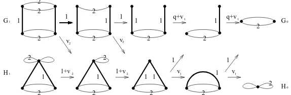
As a common strategy in computing the multivariate Tutte polynomial of any graph, the duality identity (11) and the deletion-contraction operations (12) are conducted repeatedly to derive the the multivariate Tutte polynomial of a cylinder graph. Using the simplest cylinder graphP1×C2 as an example, we first illustrate the basic process in conducting the deletion-contraction operations on cylinder graphs with two types of edges. Figure 4 illustrates how the two different types of edges affect the operation. Note that we use wide and dark lines to draw type 1 edges (paths), but lighter and thinner lines to draw type 2 edges (cycles). For each edge that is being operated, we put a number 1 or 2 besides it to indicate the edge type. Each arrow represents one of the Tutte polynomial operations in (12), and the label above the arrow is the coefficient of the operation. In this system of graphs, the multivariate Tutte polynomial of any graph equals to the sum of the multivariate Tutte polynomial of the next directed graph times its coefficient.
2
2 2
G
H
G
H
1
1
0
0
2 2
2 2 2
2 1
1
1 1
1 1
1 1
1 1+v v1
v
q+v1
2
1
1 2
2
2
2
2
1 1 1
v
2
2
2 1+v2
q+v1
v1
Figure 4: An Example of Operations on CylinderP1×C2
of such graphs. From Figure 4, one can see clearly that
Z(G1;q,v)
Z(H1;q,v)
=
1 v2 0 1+v2
2
q+v1 0 1 v1
2
Z(G0;q,v)
Z(H0;q,v)
. (21)
This shows that there is a recursive relation between the multivariate Tutte polynomials of the family of graphs{Fn,2; n≥1}. For cylinder graphs Pn×Ckwith largerk, a similar but more complicated recursive relation exists in a family of graphsFn,k, which includes more graphs and will be defined precisely shortly. Similar toFn,2, as shown in Figure 4, the graphs inFn,k are different from each other only at leveln. In fact, these subgraphs on the leveln, a special kind ofcap graphs(defined in Appendix 5), are found to have a one-to-one relationship with noncrossing partitions of the vertices ofCkin[HL07].
A noncrossing partitionΓof the vertices V ={0, ..,k−1}ofCk, is a partition in which the convex hulls of different blocks are disjoint from each other, i.e., they do not "cross" each other. It was first introduced in[Kre72]and shown to be counted by Catalan numbers. Now the family Fn,k can be defined as
Fn,k={Γ(n,k):Γis a noncrossing partition ofCk}, (22)
whereΓ(n,k)is obtained by conflating vertices of subgraph at levelnof the cylinder graph Pn×Ck according to the set of blocks inΓ. Thus a loop is created if two vertices are in the same set of blocks inΓ. For example, given partitionΓ ={{0, 1}}, Γ(1, 2)is the same asH1 in Figure 4. Actually, the graphΓ(n,k)is a special kind ofcapped cylinder graph, which is defined in Appendix 5.
In addition, letG be an ordering of the noncrossing partitions ofCkand define
Z(n;q,v) = [Z(Γ(n,k);q,v)]G, (23) which is the column vector of the multivariate Tutte polynomial of the graphs inFn,krelative to the ordering ofG. Then similar to equation (21), a general recursive relation can be obtained as the following:
Theorem 5. For each n≥1, and the edge lengthsv={v1, v2},
Z(n;q,v) =A(q,v)Z(n−1;q,v) =An(q,v)Z(0;q,v), (24)
where the transfer matrix
Note thatΘ, ∆, M, and B are matrices defined for noncrossing partitions, which will be defined precisely in formulae (39)-(43) in Appendix 5. The proof of this theorem goes along the same line with the proof of Theorem 4.2 in[HL07], but is more complicated since path and cycle edges in the cylinder graph are considered to be of two types with different length distributions. The details of the proof require precise identification of various quantities, see Appendix 5. To demonstrate the use of Theorem 5, we show two examples of evaluating the multivariate Tutte polynomial of the cylinder graph in the appendix.
4.2.2 Exact Values of the Expected Lengths of MSTs of Cylinder Graphs
In this section, we study the expected lengths of MSTs for cylinder graphs with different edge length distributions on different types of edges, thereby extend the results in [HL07]. By applying the generalized formula (4) and the multivariate Tutte polynomial (24) in the previous section, both exact values and asymptotic behaviors of the expected length of MST for the cylinder graphs are investigated. While the exact value property is the focus of this section, the asymptotic behaviors are discussed in the next.
For the simplicity of notation, we letGn,k=Pn×Ck. In the following, the edge length distributions on type 1 (path) and type 2 (cycle) edges are denoted asF1andF2respectively. Similar to the notations used in Section 4.1.2, for specialized distributions F1 and F2, we denote the expected lengths of MSTs of cylinder graphs asELeu
M S T(Gn,k), if F1 ∼exp(1) and F2 ∼ U(0, 1), and as ELueM S T(Gn,k), if
F1∼U(0, 1)andF2∼exp(1).
Proposition 2. For the cylinder graph Pn×Ck,
ELeu
M S T(Gn,k) =n
e−k k −1+
Z 1
0
(1−t)(n+1)ke−nktZq(Gnk; 1,v(t))dt,
wherev(t) ={v1(t),v2(t)}, v1(t) =et−1and v2(t) =t/(1−t).
ELue
M S T(Gn,k) = Z 1
0
e−(n+1)kt(1−t)nkZq(Gnk; 1,u(t))dt
−1+ke
−(n+1)
n+1 + 1
n+1 k X
i=1
(1−e−(n+1))i−1
i , (26)
whereu(t) ={u1(t),u2(t)}, u1(t) =t/(1−t), and u2(t) =et−1. Zq(Gnk; 1,u(t))is the derivative of the multivariate Tutte polynomial of the cylinder graph Pn×Ckwith respect to q.
Proof:
Case 1: IfF1∼exp(1)andF2∼U(0, 1), then by the general formula (4) we have
ELeu
M S T(Gn,k) = Z 1
0
(1+v2(t))−(n+1)k(1+v1(t))−nkZq(Gnk; 1,v(t))−1
dt
+
Z ∞ 1
1 1
2 1
2 1
2
1
1 2
2 2
2 2
2 2
2 2
1 1
1 1
1 1
1
1
1 1
G24 G24′
Figure 5: An Example ofP2×C4 with Contracted Cycles
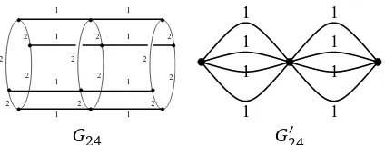
where v(t) = {v1(t),v2(t)}, v1(t) = et−1 , v2(t) = t/(1−t) and the graph G′nk is obtained by contracting the edges on all the cycles inPn×Ck. An example ofG′24is pictured in Figure 5. By formulae (10) and (13), it is not hard to check that
Z(Gnk′ ;q,v) =q(q+ (1+v1)k−1)n, and
Zq(G′nk; 1,v) = (1+v1)nk+n(1+v1)k(n−1). Hence forv1(t) =et−1, the second integral in formula (27) ofELue
M S T(Gn,k)can be computed easily as
Z ∞ 1
e−nkt(enkt+ne(n−1)kt)−1 dt=ne
−k
k .
Hence the first part of Proposition 2 is proved.
Case 2: IfF1∼U(0, 1)andF2∼exp(1), we have
ELue
M S T(Gn,k) = Z 1
0
(1+u2(t))−(n+1)k(1+u1(t))−nkZq(Gnk; 1,u(t))−1
dt
+
Z ∞ 1
(1+u2(t))−(n+1)kZq(Gnk′ ; 1,u(t))−1 dt, (28)
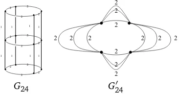
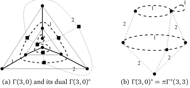
whereu(t) ={u1(t),u2(t)},u1(t) =t/(1−t),u2(t) =et−1. Note that we useu(t)to denote the edge weight vector in this case, in order to differentiate it with the one in case 1. The graphGnk′ is obtained by contracting the edges on all the paths inPn×Ck. More precisely,Gnk′ becomes(Ck)n+1 with type 2 edges, that is a k-cycle with n+1 parallel edges on each side. An example of G24′ is pictured in Figure 6.
While the standard Tutte polynomial ofGnk′ for anynmay be complicated to compute directly, the multivariate Tutte polynomial is much easier to obtain. This is largely due to the parallel-reduction identity (13) of the multivariate Tutte polynomial. The contracted graphGnk′ may be considered as a cycleCkwith weightu= (1+u2)n+1−1 for every edge. In addition, sinceu2(t) =et−1, we have
u(t) =e(n+1)t−1.
One can check that the multivariate Tutte polynomial ofCkwithu=ue for every edgeeis
Z(Ck;q,u) = (q+u)k+ (q−1)uk.
Therefore,
1
1 1
1 1 1
1 1 2 2
2 2 2 2
2 2
2
2 2 2
2
2 2
2 2 2
2
2 2 2
2 2
G24 G′24
Figure 6: An Example of P2×C4with Contracted Paths
Thus
Zq(G′nk; 1,u(t)) =ke(k−1)(n+1)t+ (e(n+1)t−1)k.
Plug these into the second integral, which we name asI2ue(n,k), in formula (28) and obtain
I2ue(n,k) =
Z ∞ 1
(1+u2(t))−(n+1)kZq(G′nk; 1,u(t))−1
dt
=
Z ∞ 1
ke−(n+1)t+ (1−e−(n+1)t)k−1 dt
= ke
−(n+1)
n+1 + Z 1
1−e−(n+1)
tk−1
(n+1)(1−t) dt,
by a change of variable.
By expanding the termtk−1, we obtain
I2ue(n,k) =ke
−(n+1)
n+1 + 1
n+1 k X
i=1
(1−e−(n+1))i−1
i . (29)
Hence the second part of Proposition 2 is also proved.
Note thatI2ue(n,k)→0, asngoes to infinity. We will use this property in calculating the asymptotic value ofELue
M S T(Gn,k)/nin the next section. Now the values ofELue
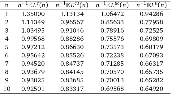
M S T(Gn,k) andELeuM S T(Gn,k)can be computed for any cylinder graph as long as its multivariate Tutte polynomial is known. In Tables 1 and 2, we compare the exact values of
n−1ELM S T(Gn,k)
for the cases of{F1(t) =F2(t) =1−e−t},{F1(t) =1−e−t andF2(t) =t},{F1(t) =t andF2(t) = 1−e−t}, and{F1(t) =F2(t) =t}. While the last case was checked in Hutson and Lewis[HL07], we use it to compare with other cases.
For the simplicity of notation, we denote
EL(n) =ELM S T(Gn,k). (30)
Note that for allnin Table 1 andn≥3 in Table 2, we have
Table 1: Exact Values ofPn×C2 for Different Edge Distributions
n n−1ELe(n) n−1ELeu(n) n−1ELue(n) n−1ELu(n)
1 1.35000 1.13134 1.06472 0.94286
2 1.11349 0.96567 0.85633 0.77958
3 1.03495 0.91046 0.78916 0.72525
4 0.99568 0.88286 0.75576 0.69809
5 0.97212 0.86630 0.73573 0.68179
6 0.95642 0.85526 0.72238 0.67093
7 0.94520 0.84737 0.71285 0.66317
8 0.93679 0.84145 0.70570 0.65735
9 0.93025 0.83685 0.70013 0.65282
10 0.92501 0.83317 0.69568 0.64920
k=2
Table 2: Exact Values ofPn×C3 for Different Edge Distributions
n n−1ELe(n) n−1ELeu(n) n−1ELue(n) n−1ELu(n)
1 2.17421 1.71031 1.82033 1.56310
2 1.64128 1.33985 1.35248 1.20091
3 1.46555 1.21652 1.20432 1.08083
4 1.37779 1.15487 1.13103 1.02083
5 1.32515 1.11787 1.08715 0.98483
6 1.29005 1.09321 1.05790 0.96084
7 1.26499 1.07559 1.03702 0.94370
8 1.24619 1.06238 1.02136 0.93084
9 1.23156 1.05210 1.00917 0.92084
10 1.21986 1.04388 0.99943 0.91284
k=3
4.2.3 Asymptotic Values of the Expected Lengths of MSTs of Cylinder Graphs
Tables 1 and 2 show that the values of ELM S T(Gn,k)/n are decreasing for all the four cases as n grows larger. Hutson and Lewis[HL07]showed that ELu
M S T(Gn,k)/nconverges to a number that can be represented by the dominant eigenvalue of their transfer matrix. For the cylinder graph with mixed edge weight distributions, we prove a similar asymptotic result in Theorem 3. Recall that Perron-Frobenius theorem says a nonnegative primitive matrix has a unique eigenvalue of maximum modulus, which is called the Perron-Frobenius eigenvalue, see Th2.1 in[Var62].
To prove Theorem 3, we first show three basic lemmas.
In particular, at q=1, the Perron-Frobenius eigenvalue of A(1,v)is
λ(1,v) = (1+v1)k(1+v2)k,
with the corresponding eigenvector as Z(0; 1,v).
Proof: To show the transfer matrix A(q,v) given in (25) is primitive, it is enough to show it is
irreducible and has all positive entries on the diagonal, see Theorem 8.5.5 in [HJ86]. Both of these two properties are easy to verify, because it is enough to show these are true for A(q,v) at
q = v1 = v2 = 1. In this case, our transfer matrix A(1,v) is reduced to the transfer matrix in [HL07]at(x−1)(y−1) =1, which was shown to be irreducible and have positive diagonal entries. In addition, since A(q,v) is clearly nonnegative, by Frobenius theorem, it has the Perron-Frobenius eigenvalue, which we denote asλ(q,v).
Since graph Γ(0,k) = (V,{E1,E2}) has edge count |E1| = 0, |E2| = k and graph Γ(1,k) = (V′,{E1′,E2′})has|E1′|=k, |E2′|=2k, from the simplification formula (8) of the multivariate Tutte polynomial atq=1, we have
Z(Γ(0,k); 1,v) = (1+v2)k,
and
Z(Γ(1,k); 1,v) = (1+v2)2k(1+v1)k= (1+v1)k(1+v2)kZ(Γ(0,k); 1,v).
Moreover, Z(1; 1,v) is a vector of Z(Γ(1,k); 1,v) for all noncrossing partitions Γ ∈ G, thus by Theorem 5,
Z(1; 1,v) =A(q,v)Z(0; 1,v) = (1+v1)k(1+v2)kZ(0; 1,v).
Therefore, Z(0; 1,v) is a positive eigenvector of the nonnegative matrix A(1,v), with the corre-sponding positive eigenvalue(1+v1)k(1+v2)k. Thus by Theorem 8.1.30 in[HJ86], atq=1, the eigenvalue of maximum modulus ofA(q,v), which is the Perron-Frobenius eigenvalue, is
λ(1,v) = (1+v1)k(1+v2)k.
This completes the proof of Lemma 2.
Next we show that
Lemma 3. For v = {v1,v2}, if we let Zq(Pn×Ck; 1,v) be the derivative of the multivariate Tutte polynomial of the cylinder graph Pn×Ckwith respect to q and evaluated at q=1, then
Zq(Pn×Ck; 1,v)
n(1+v2)(n+1)k(1+v 1)nk
→ λq(1,v)
λ(1,v) , as n→ ∞.
Proof: The proof of this lemma goes along the similar line as the proof of Theorem 7.1 in[HL07].
Adopt the notations there, we let ξ(q,v)be the Perron-Frobenius eigenvector. Choose a scaling of
ξ(q,v)such thatξ(1,v) =Z(0; 1,v). If we let
r(q,v) =Z(0;q,v)−ξ(q,v), then
Z(n;q,v) = An(q,v)Z(0;q,v) =An(q,v)(ξ(q,v) +r(q,v))
Therefore, by taking derivative on both sides of equation (31) with respect toq,
Zq(n;q,v) = nλn−1(q,v)ξ(q,v)λq(q,v) +λn(q,v)ξq(q,v) +nAn−1(q,v)r(q,v)Aq(q,v) +An(q,v)rq(q,v).
We are only interested in the above quantity atq=1, at whichξ(1,v) =Z(0; 1,v)andr(1,v) =0. This shows that, by dividingnλn(1,v), we obtain
Zq(n; 1,v)
nλn(1,v) =
λq(1,v)
λ(1,v) Z(0; 1,v) +
ξq(1,v)
n +
A(1,v)
λ(1,v)
n r q(1,v)
n .
Asn→ ∞, obviouslyξq(1,v)/n→0. Since the matrixA(q,v)is primitive
A(1,v)
λ(1,v)
n
→D(1,v), asn→ ∞,
for some matrixD(1,v), according to Theorem 8.5.1 in[HJ86]. Hence
A(1,v)
λ(1,v)
n r q(1,v)
n →0, asn→ ∞.
Consequently,
Zq(n; 1,v)
nλn(1,v) →
λq(1,v)
λ(1,v) Z(0; 1,v), asn→ ∞.
SinceZq(n; 1,v)is a vector of Zq(Γ(n,k); 1,v)for allΓ∈ G, we have for any noncrossing partition
ΓofCk,
Zq(Γ(n,k); 1,v)
nλn(1,v)Z(Γ(0,k); 1,v)→
λq(1,v)
λ(1,v). asn→ ∞.
If Γ is the partition consisting of k isolated vertices, then Γ(n,k) is the cylinder graph Pn×Ck
and Γ(0,k) is the cycle Ck with only type 2 edges. Therefore, by Lemma 2 and the fact that
Z(Ck; 1,v) = (1+v2)k, Lemma 3 is proved.
Now by dominated convergence theorem, Theorem 3 follows easily from the next lemma, details are omitted.
Lemma 4.
0< Zq(Pn×Ck; 1,v)
n(1+v2)(n+1)k(1+v1)nk
≤ (n+1)k
nk .
Proof of Lemma 4:Let the edge subsetA=A1∪A2, where the setA1,A2consists of type 1 and type
2 edges inArespectively. By the definition of the multivariate Tutte polynomial,
Z(Gnk;q,v) =X
A⊆E
qk(A)v|A1|
1 v |A|−|A1|
2 ,
where 0≤ |A1| ≤nkand 0≤ |A2| ≤(n+1)k.
As such, by taking derivative on both sides of the above,
Zq(Gnk;q,v) =X
A⊆E
k(A)qk(A)−1v|A1|
1 v |A|−|A1|
then
Since the number of components in a graph is bounded by the number of vertices the graph has, for the cylinder graphPn×Ck,
which completes the proof of Lemma 4.
Theorem 3 shows that to calculate the asymptotic value ofELM S T(Gnk)/nfor a specific value ofk, one only needs to findλq(1,v). The calculation ofλq(q,v)in general is hard, since we do not have enough information forλ(q,v) at q 6= 1. However, following the idea of using the characteristic polynomial ofA(q,v)mentioned in[HL07], one can find the following without much difficulty
λq(1,v) =−Pq(λ(1,v); 1,v)
Pλ(λ(1,v); 1,v), (33)
where P(λ;q,v) is the characteristic polynomial ofA(q,v), Pq(λ(1,v); 1,v)and Pλ(λ(1,v); 1,v) are
obtained by taking derivative of P(λ;q,v) with respect to q andλ respectively, then evaluated at
q=1.
Finally, recall that we usedEL(n)as a shorthand for ELM S T(Gn,k)in (30), where Gn,k denotes the
cylinder graph Pn×Ck. With the calculation of the transfer matrix for k = 2, 3 at the end of Section 4.2.1, we compute the asymptotic values ofn−1EL(n)by applying Theorem 3 and formula
(33). The results are shown in Table 3.