Intergenerational Economic Mobility
in the United States, 1940 to 2000
Daniel Aaronson
Bhashkar Mazumder
a b s t r a c t
We estimate trends in intergenerational economic mobility by matching men in the Census to synthetic parents in the prior generation. We find that mobility increased from 1950 to 1980 but has declined sharply since 1980. While our estimator places greater weight on location effects than the standard intergenerational coefficient, the size of the bias appears to be small. Our preferred results suggest that earnings are regressing to the mean more slowly now than at any time since World War II, causing economic differences between families to become more persistent. However, current rates of positional mobility appear historically normal.
I. Introduction
Is the United States a less economically mobile society than it was a half-century or more ago? Have economic and policy changes over this period changed the impact of parental influences in determining one’s future earnings? These questions have a long and notable history in the social sciences, as well as in popular discussion. Recent attention may be partly driven by studies over the past 15 years (for example, Solon 1992; Mazumder 2005) demonstrating that income
Daniel Aaronson is an economic advisor in the economic research department at the Federal Reserve Bank of Chicago. Bhashkar Mazumder is a senior economist in the economic research department of the Federal Reserve Bank of Chicago and executive director of the Chicago Census Research Data Center. The authors thank Merritt Lyon for excellent research assistance. They are especially thankful to Tom Hertz who offered several very helpful suggestions. They also acknowledge Anders Bjo¨rklund, Kristin Butcher, John DiNardo, Greg Duncan, David Levine, Bruce Meyer, Gary Solon, Dan Sullivan, Chris Taber, and seminar participants at several conferences and universities. The views presented here are not necessarily those of the Federal Reserve Bank of Chicago or the Federal Reserve System. The data used in this article can be obtained beginning August 2008 through July 2011 from Bhashkar Mazumder, Research Department, Federal Reserve Bank of Chicago, 230 S. LaSalle St, Chicago IL 60604, bmazumder@frbchi.org.
[Submitted June 2006; accepted March 2007]
ISSN 022-166X E-ISSN 1548-8004Ó2008 by the Board of Regents of the University of Wisconsin
System.
persists across generations at a far higher rate than previously believed by economists (for example, Becker and Tomes 1986) and, perhaps, the public.1
Most studies have measured intergenerational income mobility at a point in time and, typically, for a limited group of cohorts. Therefore, it is unclear whether current estimates of mobility have characterized the U.S. economy for some time. The few studies that have examined long-term trends in intergenerational mobility (Mayer and Lopoo 2005; Hertz 2007; Lee and Solon 2006)2suffer from two basic data short-comings. Namely, the intergenerational samples that they use do not go very far back in time and are based on small samples. Given the pronounced changes in inequality and the returns to schooling over the century, it is important to have reliable esti-mates of mobility for more than just the most recent decades. Moreover, small sam-ple sizes make it difficult to identify precise trends in the time-series.
In addition to filling an important void in the literature, greater knowledge of trends in intergenerational mobility can potentially lead to a deeper understanding of the underlying mechanisms by which income is transmitted across generations. The development of a time series on intergenerational mobility provides a source of variation for researchers to exploit to improve our understanding of intergenera-tional linkages. For example, Solon (2004) extends the Becker-Tomes model and shows that intergenerational mobility is driven by factors that have undergone di-verging trends. All else equal, the fact that the returns to human capital have risen in recent decades (Katz and Autor 1999; Goldin and Katz 1999) implies that inter-generational mobility should have fallen.3On the other hand, the emergence of the
Great Society programs in the 1960s (for example, food stamps, WIC) and the de-segregation of schools should have fostered greater equality of opportunity. How these countervailing trends have impacted changes in intergenerational mobility is ultimately an empirical question.
In this paper, we take advantage of the large samples available in the decennial Censuses. Because parents and children cannot be linked across Censuses, we em-ploy an approach analogous to a two-sample instrumental variables (TSIV) estimator to develop a consistent intergenerational mobility series back to 1940.4Our primary approach uses state of birth to match adult sons’ earnings with the income of
1. Both theNew York TimesandWall Street Journalprinted a series on economic mobility in May and June of 2005. The New York Times articles can be found at http://www.nytimes.com/pages/national/class/. The initialWSJarticle is at http://www.post-gazette.com/pg/05133/504149.stm (theWSJsite is subscription only). The public’s beliefs are described in a New York Times poll asking ‘‘Is it possible to start out poor, work hard, and become rich?’’ (http://www.nytimes.com/packages/html/national/20050515_CLASS_ GRAPHIC/index_04.html) The share answering affirmatively increased from 60 percent in 1983 to 80 per-cent in 2005. The General Social Survey also asks about social mobility (Questions 1058 and 1059). Although the questions are somewhat ambiguous, they suggest little change, and perhaps a slight improve-ment, since the mid-1980s in the belief that upward mobility is possible.
2. Related, there is a large literature, primarily in sociology, on intergenerational occupational mobility. Ferrie and Long (2005), for example, compares intergenerational occupational mobility during the second half of the 19thand early 20thcenturies to estimates derived from modern data sets, such as the National Longitudinal Surveys.
3. A constant relationship between parent income and children’s schooling would lead to a stronger inter-generational association in income if the returns to schooling rise.
synthetic families, developed from the age of their children and their state of resi-dence, in a previous generation. This estimator is roughly equivalent to using dummy variables for state of birth as instruments for parental income.
Our measure of economic mobility is based on the relationship between adult men’s log annual earnings and log of annual family income in the previous genera-tion. This regression coefficient, commonly known as the intergenerational elasticity (IGE), describes how much economic differences between families persist. Since the IGE measures quantitative movements across the income distribution, it can be used to ask questions such as how quickly families can move from the poverty level to the mean level of income. Our preferred estimates of the IGE suggest that economic mo-bility was relatively low in 1940 but increased over the subsequent four decades. However, economic mobility fell sharply during the 1980s and failed to revert, per-haps even continued to decline, in the 1990s.
We also produce estimates of the IGE that include birth cohort effects and find that mobility has declined for more recent birth cohorts, especially men born in the late 1950s and the 1960s. These time patterns may partly reconcile the results from pre-vious studies that have used different birth cohorts observed in different decades (for example, Altonji and Dunn 1991; Solon 1992; Mazumder 2005; Bratsberg et al.
2007), although we certainly acknowledge that differences across surveys and econo-metric methodology play a key role as well (Mazumder 2005).
We explicitly show that trends in the IGE are similar to those in cross-sectional inequality over the 20th century (Katz and Autor 1999; Piketty and Saez 2003). As a brief example, wage dispersion, as measured by the difference in the 90th and 10th percentiles of men’s hourly wages, fell during the great wage compression of the 1940s and rose sharply between the late 1970s and mid 1990s (Katz and Autor 1999). That this pattern has similarities to our estimates of intergenerational mobility is not wholly surprising. Cross-sectional measures of inequality provide a ‘‘snap-shot’’ of inequality at a moment in time while measures of intergenerational persis-tence of inequality provide one version of a ‘‘moving picture.’’ It could be that the same underlying factors that lead to changes in traditional measures of short-term inequality, such as changes in the returns to skill, also result in changes to long-term inequality measures. In fact, the time pattern in the returns to education bears a strik-ing resemblance to our measure of intergenerational persistence. Nevertheless, years of schooling only partly explains the time pattern in the IGE. We find, for example, that even after accounting for changes in the return to education that the IGE is sig-nificantly higher after 1980.
Some researchers prefer to use the intergenerationalcorrelation(IGC) rather than the IGE as a measure of intergenerational mobility. In principle, the two measures could show different time patterns. The IGC is roughly a measure ofpositional mobil-ity, the likelihood an adult son moves position in the income distribution relative to his parent’s place a generation prior. An IGC of 1, for example, implies that a child’s position in the income distribution perfectly replicates that of their parent’s in the prior generation. That is, there is no intergenerational mobility in rank or position.
We find that the IGE’s time-series pattern differs from the IGC, particularly prior to 1980. Consequently, how we think about the decline in intergenerational mobility exhibited by both the IGE and IGC during the 1980s depends to a degree on which measure is emphasized. The IGC suggests that the 1980s change is a return to earlier,
pre-1970s, norms. By contrast, the high rate of intergenerational income persistence exhibited by the IGE in the 1980s and 1990s may reflect a more pronounced change from the rest of the post-WWII period. Accordingly, at the close of the twentieth cen-tury, the rate of positional movement of families across the income distribution appears historically normal, but, at the same time that cross-sectional inequality has increased, earnings are regressing to the mean at a slower rate, causing economic differences between families to persist longer than they had several decades ago.
Finally, it is important to highlight that our two-sample estimator likely produces an upward biased estimate of the IGE. This bias may be large if state-specific factors—such as differences in endowments,5policies, cost of living, or local neigh-borhood, school, or peer conditions related to state of birth—are a large part of what the IGE measures.6Therefore, our estimates may exaggerate the importance of birth-location factors relative to the traditional IGE, which places less, although still pos-itive, weight on these factors. However, for more recent decades, we use a separate identification strategy that purges our estimate of state-level geographic effects and find very similar trends. This exercise reveals that the effects of state-specific factors are not large enough to account fully for the decline in mobility we identify in recent decades and for more recent birth cohorts. This finding should not be taken to mean that there are no effects on the IGE arising from the public provision of investment in human capital as in Solon (2004). Rather, any variation arising from state differences in public investment have not had meaningful effects on our estimates of the trend in the IGE. Similarly, results based on the Panel Study of Income Dynamics (PSID) and National Longitudinal Survey of Youth (NLSY) also indicate that the state-specific effects are relatively small compared to the overall IGE, although these results are less conclusive due to the small samples used.7We also explicitly show that state cost-of-living differences are not an important explanatory factor.
Regardless of the size of the bias, our broader descriptive measure is still informa-tive about trends in the importance ofaveragefamily income in one’s state of birth on children’s economic success. Although strictly speaking, this alternative measure should be given a different interpretation than the IGE, our results still provide one useful gauge of intergenerational mobility.
II. Empirical methods
The standard statistical model of intergenerational income mobility relates a child’s (usually son’s) permanent log income or earnings,yi, to his parent’s
(usually father’s) permanent log income,Xi:
5. These could include differences in physical capital or agglomeration effects, which may be autocorre-lated over time. Since children tend to stay in their birth state, persistent state differences in factors of pro-duction will bring about an association between parent’s and their adult children’s productivity and hence income. We consider the parent’s residential choice, which encompasses these factors, to be one aspect of the intergenerational transmission process.
6. It is important to emphasize that the traditional IGE measure is not a causal estimate of the effect of parent income on children’s earnings but rather captures all factors (including birth-location factors), that are correlated with parent income and children’s future earnings.
yi¼a+rXi+fðchild0s ageÞ+fðparent0s ageÞ+ei
ð1Þ
Since each generation’s income measure is expressed in logs,ris the intergenera-tional elasticity (IGE). Equation 1 is left intenintergenera-tionally sparse so thatrcaptures the full association between the parent’s economic status and their children’s later out-comes. So, for example, any effect related to birth location that is correlated with
Xiwill be included inr. The only controls typically included are the age at which
income is measured in each generation in order to control for life-cycle effects. It is now well established (Solon 1992) that a consistent estimate ofrmust account for measurement error in parent permanent income. In practice,Xiis usually proxied
by multiyear averages in order to smooth out the transitory component of earnings.8 Furthermore, Haider and Solon (2006) show that, as a result of heterogeneous pat-terns in life-cycle earnings profiles, OLS and IV estimates may be inconsistent due to the age at which thechild’searnings are measured. They find that estimates are biased downward (upward) when the income of the children is measured at a young (old) age. The bias is minimized around age 40.
Our goal is to estimate a time-series ofr.We begin with a regression equation that is similar in spirit to Lee and Solon (2006), in that it offers a time-varying estimate of the intergenerational elasticity while also addressing various statistical issues identi-fied in the literature. Our most complete specification is:
yibst ¼a+g1tðage-40Þ+g2tðage-40Þ
where the dependent variableyibstis the log annual earnings of childi, born in birth
co-hortb(measured in five year bands), in states, at timet. The key independent variable is
Xibs, the log of family income for individualiborn in birth cohortband states.
Following Lee and Solon (2006), we address the problem of bias stemming from het-erogeneous age-earnings profiles by interacting parent income with a quartic in sons’ age minus 40 (d1tod4)9. Other coefficients on parent income will then reflect effects
for 40-year-olds. We also control for year effects (ut), cohort effects (vb), and for a
quar-tic in child’s age (minus 40) that might affect thelevelof earnings. Unlike Lee and Solon, we allow for this age profile to vary by year (g1ttog4t) because the age-earnings
profile is likely to have changed substantially over the time period we are analyzing.10 In order to measure changes in intergenerational mobility over time, we include additional terms involving parent income. One way to measure time trends in the IGE is simply to include an interaction between parent’s income and the outcome year.
8. Mazumder (2005) shows that long time averages are needed to fully solve the problem. Other approaches have used instrumental variables (Solon 1992; Zimmerman 1992) or method of moments (Altonji and Dunn 1991; Zimmerman 1992).
9. More recently, Bo¨ hlmark and Linquist (2006) have found changes over time in the pattern of the life cycle bias in Sweden. We found that our results are barely affected by including these interaction terms suggesting that lifecycle bias is not much of an issue in our sample.
10. For example, Altonji and Williams (2005) find that the combined returns to tenure and experience in-creased somewhat over time, especially during the 1980s.
In this specification, the time trend is captured by the coefficientrt. Changes in the IGE
by outcome year may not only reflect the effects of childhood investments but also will capture how those payoffs change over time. Therefore, for example, the same invest-ment in human capital may produce different payoffs in the labor market if the labor market returns to skill are rising over this period, as has been well documented.
Alternatively, one may want to think about how intergenerational mobility differs across birth cohorts that were exposed to different amounts of provision of public investment. For example, cohorts eligible for the GI Bill had greater access to higher education and may therefore exhibit greater intergenerational mobility. In this case, we would want to focus on trends across birth cohorts viewed in all available outcome years. We measure the cohort trendbb, by interacting parent’s income with birth
co-hort. Finally, in our most flexible specification, we includebothcohort and year inter-actions simultaneously as shown in Equation 2. In this case, we must combine the cohort and year estimates to produce meaningful estimates of the IGE for a particular cohort observed in a particular year.11While the most appropriate specification may depend to some extent on which question is being asked, we view this last specification as generally the most preferred because it accounts for both types of effects and addresses both of the leading reasons for why mobility may have changed.12
It is worth noting that while a full specification of cohort, age, and year interac-tions with parent income is typically unidentified, our strategy assumes that the age interaction with parent income is smooth and can be parameterized by a polyno-mial interacted with year.13We also smooth birth cohort effects by using five-year
categories. Nevertheless, we find that excluding any one of the three (age, cohort, or year) sets of covariates does not change our inferences about the time patterns.
Unfortunately, as we discussed earlier, it is not possible to estimate a time-varying IGE over very long periods with existing matched parent-child data sources.14Instead, we use an IV-based strategy that allows us to take advantage of the large cross-sectional
11. To implement Equation 2, we exclude one cohort interaction and one year interaction with parent in-come for identification.u, the coefficient on parent income, measures the IGE for this omitted group. The
bbandrtmeasure differences in the IGErelativeto this group. Specifically, in order to measure the IGE in
yeartfor a 40-year-old born in yearb, we must add the relevantbbandrttou. In specifications that exclude cohort (or year) interactions with family income, we drop theuXibsterm and include the full set of year (or
cohort) interactions with family income.
12. Hertz (2007) includes a nice discussion of IGE estimates based on cohort or year effects and under what conditions they produce identical results.
13. This strategy has been used in previous studies in order to identify cohort health effects (Almond and Mazumder 2005). In order to implement it, however, the same cohorts must be observed in multiple survey years; otherwise, the linear term in age would be perfectly collinear with the cohort and year dummies. Specifically, we identifyinteractionsof family income with five-year birth cohort categories, a quartic in age, and year dummies. We employ a similar approach (controlling for a smooth function of age interacted with survey year) in order to include cohort and year dummies as controls on thelevelof son’s earnings. See Bruguviani and Weber (2003) for a discussion of alternative strategies to simultaneously identify cohort, age and year effects.
samples of the decennial Census and use nonlinked parent-child data, to identify the time-varying parameters in Equation 2. IV is a common way to deal with the measure-ment error problem induced by using short-run earnings of the father. Instrumeasure-ments, typ-ically based on the status of the father,15 are consistent if the instruments are
uncorrelated with the error term in the son’s income regression. However, even if the instruments are correlated with the error term, if the direction of the bias and its magnitude is constant over time, then IV can be used to measuretrendsin the IGE.
We use an approach that is analogous to the two-sample IV (TSIV) estimator. The innovation behind TSIV, derived and originally applied in Angrist and Krueger (1992) and Arellano and Meghir (1992), is that independent data sets can be com-bined for IV estimation, so long as the instrument is in each. Dearden, Machin, and Reed (1997), Bjo¨ rklund and Ja¨ntti (1997), and Dunn (2003) specifically apply the methodology to IGE regressions as a way to overcome the lack of data matching parents and children.16In these studies, an initial data set is used to establish the re-lationship between father’s status (for example, occupation) and father’s current in-come. These estimates are used in a second data set to predict father’s permanent income based on his status. Therefore, even though neither data set includes both son’s and father’s income,r is still, under reasonable assumptions (see Bjo¨ rklund and Ja¨ntti 1997), consistently estimated.
The Census data that we rely on does not contain linked son and parent earnings or potential instruments like parental education or occupation. However, we make use of the fact that the Census has always reported state of birth. Therefore, in principle we can use this information from an earlier Census to run a first-stage regression that predicts log parental income:
Xibs¼fbs+yibs
ð3Þ
wherefbs is a vector containing a complete set of state dummies. The predicted
value from this regression,Xbs, is the average log income of parents with children
in birth cohortb, born in states. In the main analysis, we calculate average family income by state of birth for the relevant cohort and Census year and take the log of this as our predicted value of parent income, rather than running TSIV using Equa-tions 2 and 3.17That is, we use child’s state of birth to associate adult children’s out-comes with theaverageparent income from the previous generation. Group averaged
15. Solon (1992) uses father’s education and Zimmerman (1992) uses father’s socioeconomic status as instruments. Solon shows that if the instrument has a positive independent effect on son’s earnings (as is presumably the case with father’s education), IV provides an upper bound estimate of the IGE. Other instru-ments include father’s occupation (Bjo¨ rklund and Ja¨ntti 1997), ethnicity (Borjas 1994; Card, DiNardo, and Estes 2000), industry (Shea 2000), union status (Shea 2000), city of residence (Bjo¨ rklund and Ja¨ntti 1997), and job loss (Shea 2000; Oreopoulos, Page, and Stevens 2005).
16. A number of other intergenerational mobility studies have used average parent income by group (for example, occupation) as a proxy for actual parent income without explicitly giving this strategy a ‘‘TSIV’’ interpretation.
17. We prefer this approach because it avoids having to drop families with zero income as a result of the log specification and also corresponds more closely to the aggregate data on state personal income per-capita, which we will use to generate a longer (than the Census) time series of the IGE. However, our results do not change appreciably if we run the first-stage regression using bottom-coded values for the cases of zero parent income. Furthermore, in the web appendix (see Footnote 7), we have run the two-stage version and the state average income version on the NLSY and PSID and find it does not impact our inferences.
income has the additional advantage of reducing attenuation bias relative to single-year parent income measures.18To represent the previous generation in our sample, we restrict the data used to computeXbsto families with children of a similar birth
year cohort to the adult child.
It is reasonable to conjecture that state of birth is associated with other location-specific factors, such as school quality or peer effects, which may have causal influences on the unobserved productivity of the child. The recent literature on neighborhood effects shows weak evidence on children’s outcomes for boys (the group focused on here), although other work on school and teacher quality suggests otherwise.19 In addition, since many adults live in their state of birth, if there are differences in state endowments (for example, physical capital) that are persistent over time, the effects of these differences also will be captured by our instrument.
It is important to point out that all of these location-specific factors are actually part of what is captured by the traditional IGE. Recall, the IGE is a descriptive sta-tistic, not a true causal estimate of the effect of parent income on children’s earnings. However, when state average income is used as a right-hand-side regressor instead of actual family income, greater weight is placed on these birth-location effects, pro-ducing biased estimates of the IGE. This can be seen in the following example,20 where we have omitted age measures and removed the birth cohort and time sub-scripts for simplicity. Assume the true model of children’s earnings is a function not only of family income,Xis, but it is also a function of average income in one’s
state of birth,Xs:
yis¼a+bXis+gXs+ei
ð4Þ
In this example, a regression of children’s earnings on family income produces the following probability limit of the traditional IGE:
b+gCovðXis;XsÞ
VarðXisÞ
¼b+gVarðXsÞ VarðXisÞ
ð5Þ
In contrast, the regression of children’s earnings on the average family income of parents in one’s state of birth produces a coefficient with probability limitb+g which is greater than b + gVarVarððXXisÞsÞ when g> 0, since Var(Xis) >Var(Xs).
Basi-cally, the averaging of family income puts more weight on the location effects than does the traditional IGE.
18. If measurement error were classical then group averaging of family income in a given year would fully eliminate the bias. However, given that parents likely face common state shocks in a given year due to busi-ness cycles we assume that our approach only reduces the bias but does not fully eliminate it. 19. See Kling, Liebman, and Katz (2007) on neighborhood effects. The evidence on neighborhood effects appears stronger for girls. Recent papers on school and teacher effects include Aaronson, Barrow, and Sanders (2007) and Rivkin, Hanushek, and Kain (2005).
In order to get a rough sense of the amount of bias and to demonstrate our ap-proach on familiar data, the web appendix (see Footnote 7) compares estimates using state averages to OLS and alternative IV estimates with the NLSY and PSID. We find no clear evidence that there is a large amount of upward bias. Moreover, in a separate exercise, we link generations by state of birth and ancestry and include state of birth fixed effects in order to purge our Census-based estimates of state-specific location effects. We find that the implied location effects are small and cannot account for the time trends. These results strongly suggest that we are primarily capturing trends in income mobility. Nevertheless, in order to be accurate, when we refer to the IGE, it should be thought of as an intergenerational measure that is comparable to the IGE but places greater weight on location-specific effects.
III. Data
To estimatebbandrt, we use the large cross-sectional samples from
the Integrated Public Use Microdata Series (IPUMS) of the decennial Censuses from 1940 to 2000, the only censuses that contain information about income. We use the 1 percent samples from 1940 to 1970 and 5 percent samples from 1980 to 2000. Since the Census asks about annual earnings in theprioryear, our IGE estimates actually refer to the years ending in 9s, like 1999, however, we refer to the Census year in this paper.
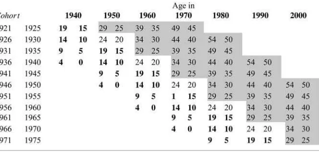
We restrict our sample to men born in the United States who had positive annual earnings in a Census year. To simulate a group of relevant synthetic families, we fur-ther restrict our sample to certain birth cohorts. These are displayed in Figure 1. Each Figure 1
Layout of Census IPUMS Data by Birth Cohort and Year
Notes: Census income data begins in 1940. Bolded area indicates years used to calculate family in-come for each cohort. Shaded area indicates years used to calculate son’s earnings.
cell represents a five-year birth cohort’s age range during a Census year. Reading across rows illustrates how cohorts age across time. In our analysis, we use cohorts for whom we can measure annual family income21when they are children (aged 0 to 19) and annual earnings when they are adults (aged 25 to 54). This has the effect of restricting our sample to men born between 1921 and 1975. The shaded area in Figure 1 represents the cohort and Census year combinations where we measure son’s annual log earnings,yibst. Our pooled sample includes over six million observations.22
For most cohorts, we measure family income by state of birth attwopoints in time and use the two-period average as our measure ofXbs.23Figure 1 bolds cells where
family income is available and illustrates how the lack of income data prior to 1940 constrains our analysis to the 1950–2000 Censuses. This is potentially an important limitation given the sharp drop in inequality that occurred during the 1940s (Goldin and Margo 1992). Therefore, in order to identify r1940 and to utilize earlier birth
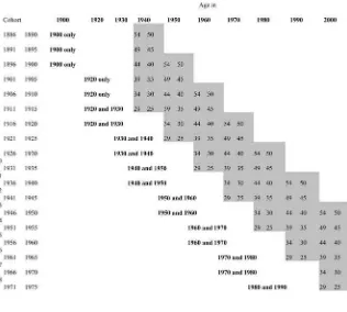
cohorts, we employ an alternative measure of family income by state, personal in-come per-capita, that is available back to 1900.24 As before, we continue to use the IPUMS to measure son’s earnings, but Figure 2 illustrates the cohorts and years that are now available to us with this second source of data. Note that per-capita income includes all forms of income collected byallindividuals residing in the state in that year, not just the self-reported income of families for our particular birth cohorts. Nonetheless, the ability to add 1940 and utilize more cohorts is valuable. In order to gauge the effects of adding data from the earlier time periods and from older cohorts we also construct a per-capita income measure for families that matches the IPUMS series by only using cohorts born after 1921 and using income data back to 1940.
As a further sensitivity check, we make use of ancestry to generate an additional source of family income variation. Since 1980, the Census has asked, ‘‘What is this
21. Following several recent studies (Chadwick and Solon 2002; Mazumder 2005; Mayer and Lopoo 2005), we chose to use family income to provide a broader measure of the impact of family resources on children’s future earnings. This allows us to abstract from questions of family structure such as changing divorce rates. In addition, for some of the earlier Censuses there are many fewer missing observations on family income than father’s income. Regardless, we have found that the results are not very sensitive to using father’s earnings instead of family income. We also make sure to remove the son’s own income from the family income measure. This makes our use of family income for sons older than age 15 less of a con-cern. For the sons, it is more meaningful to focus on earnings since conceptually, earnings capacity like skills and effort cannot be transferred from parents to kids, say, the way a house or a financial asset can. 22. Summary tables of the sample are available upon request.
23. For example, for men born in Kentucky between 1946 and 1950, we average the mean income of fam-ilies with boys between the ages of zero and five in Kentucky in the 1950 Census with the mean income of families with boys between the ages of 10 and 14 in Kentucky in the 1960 Census. We also ensure that the boys in these families were born in Kentucky. This restriction avoids problems associated with interstate migration, as discussed in Card and Krueger (1992). Family income for the 1921–25 and 1926–30 cohorts are only measured in the 1940 Census. In a robustness check we also use just asingleyear of family income measured when the children are between the ages of zero and nine alleviating concerns related to using older sons who are living at home.
person’s ancestry?’’ We match sons, whose earnings are observed in the 1980–2000 Censuses, to parents whose place of birth or whose parent’s place of birth (grandpar-ent), indicate the same ancestry. The ancestry and place of birth codes are grouped by geographic similarity to create a set of 47 distinct classifications.25The interaction of state of birth and ancestry will be used as an alternative instrument for family income Figure 2
Layout of Personal Income Per Capita (PIPC) Data by Birth Cohort and Year
Notes: Bolded area indicates years used for state PIPC for parent generation. Shaded area indicates years used to calculate son’s earnings.
25. The classifications and the mapping to the Census codes are available upon request. The Census stop-ped asking parent’s place of birth after 1970, so we are limited to measuring family income from 1940 to 1970 and to cohorts born between 1925 and 1970. Although respondents are allowed to answer more than one ancestry, we use only the first response. Ancestry is not a precisely defined term, so it is not clear how many generations back one should go. Given data availability, we can only use information about the coun-try of birth of parents or grandparents in the previous generation. For a variety of reasons, Lieberson and Waters (1988) and Fairlie and Meyer (1996) contend that the Census ancestry questions are problematic, particularly in 1980. Consequently, Fairlie and Meyer limit their analysis to those groups that give the most reliable replies—non-Europeans, Blacks, and Hispanics who provide a single ancestry response. We find similar results if we restrict our analysis to a similar subsample.
and allow us to include state fixed effects thereby purging our estimates of any birth-location effects.
IV. Results
Table 1 reports IPUMS-based results of the IGE. The first column presents a time invariant version (bbandrtare set to 0) for the 1950–2000 period.
That estimate is 0.43 (with a standard error of 0.03). Column 2 shows how the results vary over time if we do not include cohort interactions (bb¼0). The IGE appears to
increase gradually from 0.30 in 1950 to 0.38 in 1980 before sharply rising to 0.52 between 1980 and 1990. The change during the 1980s is highly significant. The IGE further increases to 0.55 by 2000, but this additional ascent is not statistically significant. In Column 3, the IGE is allowed to vary by birth cohort but not year (rt¼0). The estimates trend upward for cohorts born between 1921 and 1955 before
spiking up sharply for cohorts born in the late 1950s and early 1960s. For men born between 1961 and 1965 the estimated IGE is 0.7. There is a drop in the IGE for the late 1960s and early 1970s cohorts, but these cohorts are observed only at very young ages, so these estimates may be biased downward despite our attempts to model the age bias. Regardless, even these estimates are higher than those for the 1920s–1940s cohorts.
Finally, in Column 4, the IGE is allowed to vary by year and birth cohort. In this specification, the IGE is the sum of the coefficient on the omitted category (the 1921– 1925 birth cohort), measured byu, and the relevant cohort (bb) and year (rt)
inter-actions with family income. To compute an overall time trend, Column 5 examines how the IGE changes for 40-year-olds by combining all of the relevant coefficients from Column 4.26Now we find that there is a decline in the IGE between 1950 and 1980, most of which occurs between 1950 and 1960, followed by a large rise in the 1980s that continues through the 1990s. For completeness, Column 6 reruns Column 2 using only 35- to 44-year-olds in each year. In this specification, cohort effects are equivalent to time effects by construction. Interestingly, the results are virtually iden-tical to what we found in Column 5, our most flexible specification.
These year and cohort trends may help reconcile previous estimates in the litera-ture that have used longitudinal data with nationally representative samples to mea-sure the father-son elasticity in earnings. For example, Altonji and Dunn (1991) use a cohort of National Longitudinal Survey (NLS) men born between 1942 and 1952 whose earnings were observed primarily in the 1970s. They find an IGE of around 0.25.27Solon (1992) used a cohort of PSID men born between 1951 and 1959 whose earnings are observed in 1984 and estimated the IGE to be around 0.4. Bratsberg et al. (2007) use the NLSY covering cohorts born between 1957 and 1964 whose
26. For example, the IGE for men in 2000 who were born in 1959 is 0.347-0.143+0.375¼0.579. For sim-plicity, we assume that the cohort effect for individuals born in 1909 and 1919 is equal to the omitted 1921– 25 cohort.
Table 1
Estimates of the IGE Using Census IPUMS Data
Full sample
Implied IGE for 40-44-year-olds
35-44-year-olds only
(1) (2) (3) (4) (5) (6)
Family income 0.433 — — 0.347 —
(0.027) (0.036)
Family income*year
1950 — 0.297 — 0.056 0.404a —
(0.041) (0.023)
1960 — 0.322 — — 0.347 0.336
(0.038) (0.034)
1970 — 0.367 — 20.039 0.336 0.331
(0.025) (0.024) (0.025)
1980 — 0.375 — 20.121 0.322 0.318
(0.025) (0.032) (0.026)
1990 — 0.522 — 20.076 0.462 0.464
(0.046) (0.058) (0.044)
2000 — 0.545 — 20.143 0.580 0.571
(0.056) (0.065) (0.058)
Family income*cohort
1921–25 — — 0.337 — —
(0.028)
1926–30 — — 0.298 0.028 —
(0.028) (0.014)
1931–35 — — 0.372 0.111 —
(continued)
Aaronson
and
Mazumder
Table 1(continued)
Full sample
Implied IGE for 40-44-year-olds
35-44-year-olds only
(1) (2) (3) (4) (5) (6)
(0.031) (0.023)
1936–40 — — 0.358 0.095 —
(0.032) (0.028)
1941–45 — — 0.453 0.200 —
(0.030) (0.032)
1946–50 — — 0.425 0.191 —
(0.036) (0.037)
1951–55 — — 0.475 0.251 —
(0.037) (0.040)
1956–60 — — 0.604 0.375 —
(0.061) (0.048)
1961–65 — — 0.694 0.478 —
(0.082) (0.065)
1966–70 — — 0.578 0.398 —
(0.073) (0.063)
1971–75 — — 0.476 0.306 —
(0.090) (0.080)
N 6,115,340 6,115,340 6,115,340 6,115,340 2,121,549
Notes: All specifications include cohort dummies, year dummies, and a quartic in age 40 interacted with survey year (1950, 1960, and 1970 have a common age profile). They also include interactions of a quartic in age 40 with family income. All standard errors are clustered by state of birth.
a. Assumes that the cohort effect for 1906–10 is equal to cohort effect for 1921–25.
The
Journal
of
Human
earnings are observed in 1995 and 2001 and estimate the IGE to be 0.54. Mazumder (2005) used the Survey of Income and Program Participation (SIPP), matched to so-cial security earnings records, for cohorts born between 1963 and 1968 whose earn-ings are observed between 1995 and 1998. He estimates the IGE to be 0.6 or higher. To be sure there are other important differences between these studies, most notably the length of the time average used to measure the permanent economic status of the parents and the age at which the parents’ and children’s earnings are measured, that have likely driven the differences across studies. However, the results here suggest that the particular cohorts and the years used are also important factors.28
It is worth noting that the trends described here are not apparent in studies that have attempted to detect either cohort or year trends using the PSID (Mayer and Lopoo 2005; Hertz 2007; Lee and Solon 2006). However, there are notable limita-tions with using the PSID to study long-term trends in mobility. The PSID only be-gan in 1968. Given standard sample selection rules in the literature, it is consequently difficult to create large enough samples to produce reliable estimates of intergener-ational mobility until the early 1980s or for cohorts born before 1950.29This is par-ticularly problematic given the large rise in the return to schooling from the late 1970s into the 1980s. Furthermore, sample sizes in the PSID are especially small for more recent cohorts and attrition bias remains a concern even if it can be addressed under certain assumptions (Hertz 2007). In contrast, there appears to be evidence of a trend when comparing cohorts and outcome years across the NLS and the NLSY as implied by the results in the studies discussed above. These studies have larger intergenerational samples than the PSID and start with nationally repre-sentative samples of families in each oftwotime periods (1966 and 1979) rather than rely on only one initially representative sample in 1968.
To go back farther in time, we next turn to results that use the state-specific per-capita income data. These are displayed in Table 2 and plotted against the IPUMS estimates in Figure 3. By adding additional cohorts and an additional year of data, we increase our sample size of adult children by about 380,000 and can produce an estimate for 1940. That estimate, at 0.67 (Column 2), is higher than any subse-quent Census year. Although, the year-specific estimates match up very well with the IPUMS-based estimates beginning in 1980, including a comparable increase be-tween 1980 and 1990, they diverge prior to that. This is apparent in Figure 3. We will examine this divergence in more detail below.
Cohort effects (Column 3) are highly pronounced very early in the century before falling for cohorts born between 1915 and 1935. Thereafter, however, the cohort ef-fect gradually rises reaching a peak of 0.68 for those born between 1961 and 1965. The pattern in the cohort effects for those born since 1921 is very similar to what we found with the IPUMS sample. When we allow for both cohort and year effects, the implied estimates for the IGE (Column 5) show a roughly similar time pattern to the IPUMS-based results. The IGE is estimated at just under 0.6 in 1940, gradually falls
28. Levine and Mazumder (2007) also report a sharp increase in sibling correlation in men’s earnings—an omnibus measure of family and community influences—between cohorts born in the 1940s who entered the labor market in the 1970s compared to cohorts born in the 1960s who entered in the 1980s.
29. Typically, studies exclude children living at home beyond age 17. Ideally we want to measure adult children’s income when they are at least in their late 20s or early 30s.
Table 2
Estimates of the IGE Using Personal Income per Capita Data
Full Sample
Implied IGE for 40-year-olds
(1) (2) (3) (4) (5)
Income per capita 0.502 — — 0.466
(0.026) (0.030)
Income per capita*year
1940 — 0.670 — 0.259 0.592
(0.027) (0.037)
1950 — 0.520 — 0.052 0.579
(0.024) (0.017)
1960 — 0.509 — — 0.512
(0.029)
1970 — 0.449 — 20.101 0.383
(0.020) (0.021)
1980 — 0.399 — 20.227 0.342
(0.030) (0.025)
1990 — 0.569 — 20.172 0.495
(0.047) (0.052)
2000 — 0.530 — 20.297 0.566
(0.060) (0.054)
Income per capita*cohort
1886–90 — — 0.617 20.180
(0.038) (0.069)
The
Journal
of
Human
1891–95 — — 0.595 20.177
(0.043) (0.064)
1896–00 — — 0.573 -0.133
(0.033) (0.052)
1901–05 — — 0.688 0.015
(0.030) (0.039)
1906–10 — — 0.658 0.061
(0.032) (0.033)
1911–15 — — 0.664 0.097
(0.030) (0.028)
1916–20 — — 0.506 0.046
(0.037) (0.020)
1921–25 — — 0.429 —
(0.023)
1926–30 — — 0.354 0.018
(0.028) (0.014)
1931–35 — — 0.438 0.129
(0.033) (0.030)
Income per capita*cohort
1936–40 — — 0.409 0.103
(0.026) (0.029)
1941–45 — — 0.518 0.241
(0.034) (0.039)
1946–50 — — 0.442 0.202
(0.034) (0.038)
1951–55 — — 0.508 0.296
(0.042) (0.038)
(continued)
Aaronson
and
Mazumder
Table 2(continued)
Full Sample
Implied IGE for 40-year-olds
(1) (2) (3) (4) (5)
1956–60 — — 0.607 0.397
(0.057) (0.045)
1961–65 — — 0.675 0.497
(0.090) (0.066)
1966–70 — — 0.491 0.380
(0.090) (0.066)
1971–75 — — 0.437 0.353
(0.083) (0.058)
N 6,501,257 6,501,257 6,501,257 6,501,257
Notes: All specifications include cohort dummies, year dummies, and a quartic in age 40 interacted with survey year (1950, 1960, and 1970 have a common age profile). They also include interactions of a quartic in age 40 with per-capita state income. All standard errors are clustered by state of birth.
The
Journal
of
Human
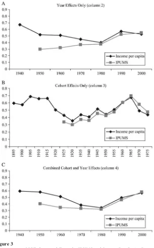
Figure 3
Comparisons of IGE Computed From the IPUMS and Income Per Capita Data
to a low of 0.34 in 1980, then rises to 0.50 in 1990 and 0.57 in 2000. As with Column 2, the estimates in Column 5 line up well with the IPUMS results from Table 1 be-ginning in 1980 but diverge a bit in the earlier decades.
There are three possible reasons for this divergence. First, per-capita income meas-ures the income of all state residents, not just the income of families in our particular cohorts. Second, since income is not asked in the Census prior to 1940, the IPUMS sample relies heavily on data from 1940 to measure family income for sons observed in the 1950s and 1960s. Since income inequality appears to be higher in 1940 relative to previous decades (see Section VI), this may have the effect of depressing IPUMS-based IGE estimates relative to per-capita income-IPUMS-based estimates.30In fact, the es-timate of the time-invariant IGE is a fair bit higher with the per-capita income sample (0.50) than with the IPUMS sample (0.43). Third, the lack of data prior to 1940 con-strains the cohorts used to estimate the IGE in the IPUMS sample. As Figure 3 shows, the cohort-specific IGEs are not very different for cohorts that are in both samples but are considerably higher for cohorts born prior to 1921 that are only in-cluded in the per-capita income sample.
In order to reconcile the estimates, we reran the per-capita income-based regres-sions using the cohorts and years available in the IPUMS. With this restricted sam-ple, we exactly match the IPUMS estimate of 0.43 when we impose a common IGE for all cohorts and years. Similarly, we used the IPUMS sample but include the fam-ily income ofallindividuals in the state and find the common IGE to be 0.52, which is close to the 0.50 estimate we obtained with the per-capita income sample. Further-more, when we define the samples similarly by imposing both data limitations, we can largely reconcile differences in the time patterns as well. Appendix Figure A1 plots the reconciled set of IGE estimates for 40-year-olds using the specification, which accounts for cohort and year effects. To be clear, we don’t view the estimates shown in this figure as representing our view of the best measure of the time trends, rather they are meant to show that the data are roughly comparable when they are both restricted in the same ways.
A. Discussion of Results
In our view, the key finding is the decline in intergenerational mobility after 1980. Our preferred set of estimates are those that use both cohort and year interactions estimated with the IPUMS data (Column 5 of Table 1). We prefer the IPUMS-based estimates since they utilize the microdata where we can clearly identify synthetic parents. We prefer the model that includes both cohort and year interactions since it allows for both leading explanations for why mobility may have changed (rising returns to skills, changing provision of public investment) to be fully reflected in the estimates. These preferred estimates imply that the IGE is higher now than at any other time in the post World War II period.
Nonetheless, we recognize that there is some uncertainty about the trends in the IGE prior to 1980 and there may be reason to think that the IGE was somewhat higher over the 1950 to 1970 period than our preferred estimates indicate. We also
have some uncertainty about the level of intergenerational mobility in 1940 and for cohorts born before the 1920s since these can only be estimated using the per-capita income data. Nonetheless, we suspect that intergenerational mobility likely increased from 1940 to 1950 based on the per-capita results. This matches the trends in cross-sectional inequality that we discuss in greater detail in Section VI.
V. Robustness Checks
Ancestry is an alternative source of variation that can be used to iden-tify the time-varying IGE. Because ancestry is not strictly tied to geographic loca-tion, it may help minimize the confounding effects of birth location. Given previous research on the potential importance of ethnic capital on wages (Borjas 1992), we begin with the presumption that averaging income by ancestry group will also produce upward biased estimates of the IGE. However, unless there have been
changes over timein the importance of ethnic capital, the use of ancestry as an
in-strument may still be informative about trends in intergenerational mobility. In our next set of results, we do just that, measuring average family income by state of birth
andancestry. Unfortunately, since ancestry is only asked since 1980 we can only im-plement this approach for the last three Censuses.
In a second specification, we also include a full set of state of birth dummies in the regression so that we can identify the effect of family income on son’s earnings using differences in ethnicity within states.31 In this specification, birth-location effects that operate at the state level are no longer captured by our IGE estimates, although any ethnic capital effects are. To be clear, this approach also removes any effects that are due to themeanlevel of state family income. Any difference be-tween estimates from a statistical model that includes state fixed effects and one that does not provides a rough indication of the size of the upward bias arising from the greater weight place on location effects. In a third specification, we also include a full set of state of birth by Census year interactions. In principle, this should absorb any changes in the state specific effects that occur over time. However, it is quite demanding on the data given all of the other controls, including year-specific age profiles and parent income by age interactions, and the more limited samples that contain ancestry.
Table 3 presents the results using our most flexible specification that includes both cohort and year interactions with family income. Recall that this model requires sum-ming up the relevant components of the IGE by birth cohort and outcome year. As before, we construct the implied IGE for a 40-year-old in each Census year. The first two columns of Table 3 show the baseline results. Column 1 indicates a statistically significant increase in the year effect of 0.09 for 1990 (relative to 1980) and no fur-ther increase from 1990 to 2000. Much larger trends are picked up by the birth cohort interactions with family income. Individuals born in the 1930s have an IGE about 0.1 greater than those born between 1926 and 1930. However, this effect rises
31. We experimented with average family income by ancestry but found the estimates quite imprecise. However, we still find the same general time pattern.
Table 3
Estimates of the IGE Using State of Birth and Ancestry as Instruments
Baseline Model IGE at age 40
State Fixed Effects IGE at age 40
State Fixed Effects with State-Year Interactions IGE at age 40
(1) (2) (3) (4) (5) (6)
Family income 0.262 0.234 0.209
(0.024) (0.022) (0.022)
Family income*year
1980 — 0.343 — 0.293 — 0.301
1990 0.085 0.696 0.085 0.629 0.005 0.564
(0.024) (0.023) (0.002)
2000 0.008 0.689 0.002 0.615 0.009 0.658
(0.036) (0.036) (0.001)
Family income*cohort
1926–30 — — —
1931–35 0.107 0.087 0.096
(0.021) (0.019) (0.019)
1936–40 0.080 0.059 0.092
(0.023) (0.021) (0.021)
1941–45 0.372 0.333 0.372
(0.038) (0.035) (0.035)
The
Journal
of
Human
1946–50 0.348 0.310 0.350
(0.038) (0.036) (0.036)
1951–55 0.350 0.313 0.360
(0.045) (0.042) (0.042)
1956–60 0.419 0.379 0.440
(0.050) (0.046) (0.046)
1961–65 0.328 0.303 0.369
(0.059) (0.055) (0.055)
1966–70 0.321 0.297 0.347
(0.061) (0.057) (0.057)
N 4,621,092 4,621,092 4,621,092
Notes: All specifications include cohort dummies, year dummies, and a quartic in age 40 interacted with survey year. They also include interactions of a quartic in age 40 with family income. All standard errors are clustered by the combination of ancestry and state of birth.
Aaronson
and
Mazumder
dramatically for cohorts born after 1940. Overall, Column 2 shows that the IGE for a 40-year-old doubles from 0.34 in 1980 to 0.69 in 1990.
Columns 3 and 4 display results with state fixed effects. We find that adding state fixed effects has virtually no effect on the year interactions with family income and reduces the cohort interactions with family income for every single cohort group by about 0.02 to 0.03. It also reduces the coefficient on family income for the omitted group from 0.26 to 0.23. The overall effect on the IGE for 40-year-olds (Column 4) is to reduce the size of the coefficients by about 0.05-0.07, but has little effect on the trend. Finally, in Columns 5 and 6 we include state of birth interacted with year. With this specification, the contributions to the IGE from the year interactions with family income are close to eliminated but it appears to accentuate the cohort effects, which are now similar to what they were in the baseline specification. Overall, however, the effects on the trend in the IGE for 40-year-olds in each Census year are relatively small. The point estimates rise from 0.30 in 1980 to 0.56 in 1990. These results are broadly consistent with Card, DiNardo, and Estes (2000).
That the trend results are so similar across different specifications suggests that the increase in the IGE during the 1980s is quite robust. While it is likely that differences in ancestry group within state have a direct impact on son’s earnings, these direct effects would have to have increased sharply over this short period to account for the observed increase. Finally, we note that comparing the specifications with and without state fixed effects provides a rough indication of how important birth-location effects could be. For example, if we drop all the year and cohort interactions and simply estimate a common IGE without state fixed effects, our estimate is 0.55. With state fixed effects, the estimate drops to 0.47 and with state-year interactions, the estimate is 0.48. This suggests that adding state fixed effects tends to lower the level of the IGE by only about 0.08. This is too small to account for the swing of 0.15 to 0.20 that we estimate for the 1980s.
We also performed a number of other checks on our results. First, we ran ‘‘pla-cebo’’ regressions, which randomly assign state of birth in place of actual state of birth. In this case, as expected, the IGE was always around 0 with no discernible time trend. Second, we experimented with adjusting our per-capita income measures for differences in the costs of living across states, as measured in Mitchener and McLean (1999), and found our point estimates were virtually unchanged. Therefore, we can exclude geographic differences in cost of living as an explanation for these time trends. Third, we reran the regressions on a sample of only Whites. We find estimates that are uniformly lower than the full-sample estimates by about 0.1 in every period and across all cohorts. This is in accord with Hertz (2005), who finds a similarly sized difference between whites and the full sample using the PSID. However, as before, we find a large jump in the IGE between 1980 and 1990 that is statistically significant.32 This suggests that our aggregate results likely are not driven by race-specific differ-ences in economic mobility that might exist.
Fourth, we find that the results are insensitive to how we handle potential issues stemming from life-cycle bias. We think that this is likely due to the fact that our sample, unlike the PSID for example, includes all age groups in most Census years. Specifically, our inferences concerning trends are robust to whether or not we include the age interactions with family income. As we showed in Table 1, the results are robust to restricting the sample to 35- to 44-year-olds. We also found this to be true if we restrict the samples to 25- to 29-year-olds, or 30- to 34-year-olds.
Finally, we tried three alternative, but reasonable, perturbations, of family income: father’s earnings rather than family income, using a single Census year rather than averaging family income over two Censuses,33and including families with zero in-come by coding them at $1,000 (in 2000 dollars). Although the point estimates were sometimes lower (as might be expected in the single year Census case), the time trends were similar in all of these cases.
It is also worth pointing out that our intergenerational model has some similarity to the statistical model estimated in the growth literature (Barro and Sala-i-Martin 1992). In the web appendix (see Footnote 7), we explain how the two models differ, explicitly showing that they produce distinct empirical trends over the last 60 years.
VI. Trends in Inequality and the Intergenerational
Correlation
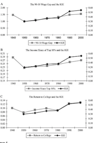
It has often been argued that economic mobility is a relevant concept for economists because an increase in mobility is thought to imply that lifetime income is more equal (Shorrocks 1978). A cross-sectional measure of inequality provides a ‘‘snap-shot’’ at a moment in time while generational mobility provides one version of a ‘‘moving picture.’’34It is especially noteworthy then that trends in generational mobility share sim-ilar patterns with cross-sectional inequality trends. For example, in Figure 4 we plot our IGE time series based on the year estimates (Table 1, Column 2) against the 90–10 wage gap as estimated by Katz and Autor (1999) and the income share of the top 10 percent as calculated by Piketty and Saez (2003).35This suggests that both traditional measures of short-term and long-term inequality tend to move together.
The comovement between these series is not wholly surprising because a change in the returns to skill could lead to a change in both the income distribution and in-tergenerational mobility. The bottom panel of Figure 4 plots the relationship between our yearly estimates of the IGE from Table 2, Column 2 against a time series of the return to college as estimated by Goldin and Katz (1999). This chart shows a clear correspondence between these measures.
33. In this case, we used family income at ages 0–9 which also addresses any concerns that our results are driven by using family income for older sons. A related concern is that there might be differential measure-ment error in family income across Census years because the sizes of the samples increase from one percent to five percent beginning in 1980. To address this potential problem, we ran the specification using family income at ages 0–9 while also dropping the 1971–75 cohort so that we never use a five percent sample to calculate family income. We found that this had no effect on our conclusions.
34. Another measure of economic mobility would be within an individual’s lifetime.
35. We use the year only estimates of the IGE here because they are more directly comparable with the time series measures in Katz and Autor (1999) and Piketty and Saez (2003) which do not in any way adjust for cohort effects.
Figure 4
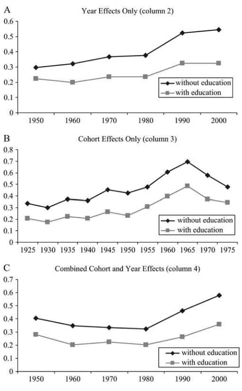
Fortunately, we can examine this proposition directly because the Census collects information on years of schooling. In order to gauge whether our IGE trends are fully accounted for by changes in the returns to schooling, we estimate our models anew with the adult son’s years of schooling as an additional explanatory variable.36Figure 5
shows the results of this exercise. We find that, in all cases, the IGE point estimates significantly decline, typically falling by between 30 and 45 percent. The time trends, however, remain visible and in some cases are quite large. For example, even when including years of education, the cohort estimate of the IGE (using the per-capita in-come sample) for those born between 1950 and 1954 is 0.22, which is less than half of the 0.48 estimate for those born between 1961 and 1965. The 1980s change in the year-specific IGE is somewhat less pronounced than before, though still statistically significant, rising from 0.24 to 0.32. Therefore, while it is clear that including edu-cation makes the changes somewhat less dramatic, the time patterns remain striking. This suggests that changes in the return to education cannot fully account for the ob-served trends in the IGE.
A related issue is that some researchers prefer to use the intergenerational
corre-lation (IGC) as a measure of intergenerational mobility because it is sometimes
thought to be immune to changes in inequality. Whether to highlight the IGE or the IGC depends on the question posed. One minus the IGE measures the degree to which earnings ‘‘regress’’ to the mean and characterizes how earnings differences between families (in percentage terms) evolve over time. Since the IGE measures quantitative movements across the income distribution it can be used to ask questions such as how quickly families can move from the poverty level to the mean level of income. Alternatively, one minus the IGC roughly measures the amount ofrank,or positional, mobility. An IGC of 1, for example, implies that a child’s position in the income distribution perfectly replicates that of their parent’s in the prior generation.
The relationship between the IGC, labeledr,and the IGE,r,is:
r¼rsparent schild
ð6Þ
wheresis the standard deviation of log income in the relevant generation. Equation 6 illustrates that ifrwere somehow ‘‘held constant,’’ trends inrandrcould differ during periods in which inequality is changing sharply. For example, in periods of rising inequality, it might be possible that the rate of movement of families across the distribution stays the same (IGC) but earnings may regress to the mean at a slower rate (IGE). In such a scenario, the IGE could be a misleading measure of rank mobility and the IGC a misleading measure of the rate of regression to the mean. We should caution the reader that there is no obvious reason to assume thatrwill stay the same when inequality changes. Further, there is no more reason to think thatr will stay constant than to assume thatrwould stay constant. In our view, it is important to report the empirical trends in both parameters and see how these parameters have
actuallychanged.
36. Specifically, we start with the three specifications used to produce our Column 2, 3 and 4 estimates of the IGE in Table 2 using the IPUMs sample. We then add years of schooling interacted with either year dummies, cohort dummies, or both year and cohort dummies. The results are plotted in Figure 5.
In principle, we can use cross-sectional inequality trends to transform our IGE estimates into correlations. Since our estimates of rt are based on pooled samples
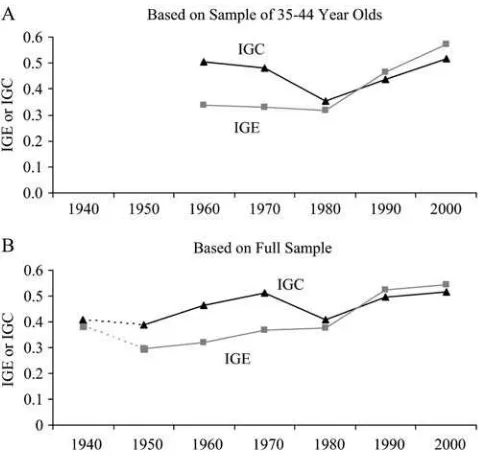
of multiple birth cohorts, family income is measured in different years, complicating the calculation of the ratio of thes’s. Consequently, we estimate the IGC using two approaches. First, we use the sample of 35- to 44-year-olds (as in Column 6 of Table 1). Here it is simple to calculate the ratio of thes’s in each generation for each year. Figure 5
The results are displayed in the top panel of Table 4 and are plotted in Figure 6.37 Our second approach uses the year-specific IGEs computed in Column 2 of Table 1. This is shown in the bottom panel of Table 4 and is based on a weighted average ofsparent
schild across all cohorts and years. This second approach is more complicated but allows us to go back to 1950 and under some assumptions produce an estimate for 1940.38
Because the across-generation inequality adjustments are large prior to 1980, we find that the IGC and IGE diverge a fair bit in the pre-1980 decades. For the sample of 35- to 44-year-olds, the IGC was essentially flat from 1960 to 1970, fell sharply between 1970 and 1980, and steadily increased from 1980 to 2000. With the full sample, the IGC, unlike the IGE, was steady or increasing during the 1940s and 1950s. With either sample, we find that the 2000 IGC was not at an especially high level by historical standards. Consequently, while intergenerational mobility unam-biguously fell in the 1980s, how we interpret this change is dependent on which mo-bility measure is the focus. Our preferred estimates of the IGE (Table 1, Column 5) that account for both cohort and year effects using the IPUMS suggests that the de-cline in mobility after 1980 represented a significant departure from the higher levels of mobility experienced post-WWII. But the IGC suggests intergenerational mobility in the 1970s was unusually high; the 1980s and 1990s were a return to a typical post-WWII level.
VII. Conclusion
We take advantage of the large samples available in the decennial Censuses and employ a two-sample estimator to develop a consistent time series
37. The trend in our parent-child inequality ratios is roughly comparable to others that can be imputed in the literature. For example, from Katz and Autor (1999), we computed the ratio of the full-time male 90/10 wage gap to the same gap 30 years prior. This generational inequality ratio fell from 1.25 in 1969 to 0.74 in 1989. They do not provide a long enough time series on the standard deviation of log wages, which is more comparable to what we do, but the 1989 generational inequality ratio is slightly higher—0.81— using this measure. A longer series can be computed from Piketty and Saez’s (2003) income share data. The gener-ational ratio of top decile income shares fell from roughly 1.4 in 1959 (and 1969) to 0.75 in 1999. While the general time pattern is the same for different measures, there are discrepancies in samples (full population versus families with young children) and measures (standard deviation of income, 90/10 wage gaps, or top income shares) that cause variation in magnitudes.
38. The 1940 computation is shown as a dashed line in figure 6 to emphasize that calculating it required several assumptions. Since we cannot estimatesparentfor 1940 (we need microdata from at least 20 years prior), we predict the 1920sparentusing the 1940 to 1990 relationship betweensparentand the share of in-come earned by the top decile of households, as reported in figure 1 of Piketty and Saez (2003). The latter series, which has a 0.96 correlation withsparent, dates back to 1920. Specifically, we ran the regression
sparent¼a + b*INCSH + e, where INCSH is the share of income earned by the top decile. The constant in this regression is 0.33 (0.09) and the slope is 1.64 (0.25). INCSH in 1920 is 0.395 andschild, calculated from the 1940 Census, is 0.914. Thus,sparentin 1940 is estimated to be 0.33 + 1.64 * 0.395¼0.977 and
sparent/schild¼0.977/0.914¼1.069. Based on Column 2 of the per-capita income results in Table 2, we as-sume the 1940 ‘‘IPUMS’’ IGE is 29 percent larger than the 1950 IPUMS estimate. Consequently, the 1940 IPUMS IGC is 0.31 (1950 IGE) * 1.29 (1940 adjustment) * 1.069 (1940 inequality ratio)¼0.43. This is similar in magnitude to the 1950 estimate, suggesting that the drop in the IGE during the 1940s is mostly driven by changes in inequality across generations.
on intergenerational mobility. Our primary approach uses state of birth to match adult sons’ earnings with the income of synthetic families from a previous genera-tion. In our preferred specification, we show that the intergenerational elasticity (IGE), a measure of how economic differences between families persist over time, fell slightly from 1950 to 1980, but rose sharply during the 1980s and may have con-tinued to rise in the 1990s. This implies that intergenerational mobility has fallen in recent decades. We also find a similar pattern across birth cohorts with mobility es-pecially low for cohorts born during the 1960s. The cohort and time trends may help to reconcile previous findings in the literature that used samples of different cohorts observed in different years. Using per-capita aggregate income data instead of micro-data from synthetic families also suggests that a decline in the IGE from 1940 to 1950 tracked the change in cross-sectional inequality.
A limitation of our strategy is that relative to the traditionally estimated IGE, our measure over-weights location specific factors such as school quality or factor endowments that are specific to one’s state of birth. However, we provide several pieces of evidence that birth-location effects have little impact on our measure of trends in intergenerational mobility of economic status. In particular, we find that when we link individuals to family income in the previous generation by both state of birth and ancestry and include state fixed effects, the implied state-location effects appear to be small. Accounting for state effects also does not affect our finding of a large drop in mobility after 1980. In any case, like the traditionally estimated Figure 6