Numerical Method for Front Tracking in Mold Filling
Modeling in Composite Injection Molding:
Non-reacting System
Mohammad Fahrurrozi1 and John R. Collier2
1)
Department of Chemical Engineering, Gadjah Mada University
2)
Emiritus Proffesor, Department of Chemical Engineering, Louisiana State University and Professor, Department of Chemical Engineering, Florida State University
Abstract
Mold filing simulation is important in mold design for liquid composite molding. Cost of commercial software for mold filling simulation is very expensive for average Indonesian companies. Therefore a more affordable simulation program is necessary to promote development of domestic technology related to liquid composite molding. This paper presents 3-dimension mold filling model based on control volume finite difference (CV-FD) numerical method on fixed grids. Front tracking was performed using volume of fluid method (VOF) implemented on CV-FD. Velocity field was computed using Darcy's equation. Computation was implemented on Fortran while contour plot were prepared using Matlab. The developed model predicts well gate pressure obtained experimentally. Since experimental data for front advancement is not available, calculation
results were compared with results for other software developed by US’s NIST. The developed model predict
front position obtain by the other software quite well.
Key words: mold filling, simulation, reaction, injection, composites
Abstrak
Pemodelan proses pengisian cetakan sangat penting untuk perancangan cetakan untuk pencetakan komposit polimer. Harga software komersial untuk simulasi pengisian cetakan sangat mahal untuk ukuran rata-rata perusahaan Indonesia. Keberadan software yang lebih terjangakau akan mendorong perkembangan teknologi domestik yang berhubungan dengan pencetakan komposit polimer. Paper ini menyajikan pemodelan pengisian cetakan komposit polimer dalam sistem 3 dimensi berbasis metoda numeris control volume finite difference (CV-FD) pada elemen yang tetap (fixed grids). Pemodelan bentuk ujung aliran polimer (front) dilakukan dengan menggunakan metoda volume of fluid (VOF). Profile kecepatan dihitung dengan menggunakan persamaanDarcy untuk sistem 3 dimensi. Perhitungan dilakukan dengan menggunakan bahasa pemrogaman Fortran dan penggambaran hasil perhitungan dilakukan dengan menggunakan Matlab. Model yang dikembangkan dapat mendekati hasil pengukuran secara eksperimen untuk tekanan pada lobang pemasukan (gate) dengan relatf baik. Karena data eksperimen perkembangan ujung aliran olimer tidak ada, maka hasil perhitungan model yang dikembangkan dibandingkan dengan hasil perhitungan dengan menggunakan software yang dikembangkan dan digunakan oleh US NIST. Software yang dikembangakn dapat memperkirakan dengan baik posisi ujung aliran polimer yang dihitung dengan menggunakan software dari US NIST.
Kata kunci: komposit, polimer, pencetakan, pemodelan
Introduction
Liquid composite molding (LCM) that includes structural reaction injection molding (SRIM) and resin transfer molding (RTM) is the most widely used to manufacturing low cost, high quality surface finish, composite (Macosko, 1989; Lindsay, 1993; Rogers, 1990, Valenti, 1992; Wilder, 1989). Growing interest in the SRIM thermosetting process was primarily driven by higher productivity and design flexibility demands in the automotive industry __________
Alamat korespondensi: Email: [email protected]
automated preform manufacturing have attracted wider SRIM and RTM applications (Lindsay, 1993; Rogers, 1990; Valenti, 1992; Wilder, 1989). The demand for SRIM and RTM parts, especially in the automotive industry, is projected to increase in the future in line with the trend of increasing non-metal content on automotive products.
In both SRIM and RTM processes, fiber preformed mats are placed inside the mold cavity prior to filling the mold with resins. The resins subsequently react and form solid structures (Macosko, 1989; Polushkinet et. al., 2002). The differences between the two processes are in the way the reaction is started and in the cycle time. While impingement mixing between two streams initiates the reaction in SRIM, a catalyst is added and sometimes heating is also required to start the reaction in RTM. Typically RTM has a longer cycle time than SRIM (Lindsay, 1993). Polyurethane (PU) formulations are the most widely used for SRIM applications while there are more variations for RTM applications. The two most important for RTM are polyester based and epoxy based formulations. With the advance of resin synthesis, the distinction between SRIM and RTM is becoming more blurred. Some chemical manufacturers have developed two component formulations that can be used for both SRIM and RTM by allowing users to adjust the curing times from the order of a few minutes (suitable for SRIM) to as high as one hour (suitable for RTM) (Lindsay, 1993). One example of this type is Xycon (urethane polyester hybrid resin) developed by Amoco (Rogers, 1990).
Mold filling is a very crucial step in both SRIM and RTM. In the short duration of mold filling, which is from the order of a few seconds to as high as only a few minutes, the resin should be able to penetrate into the mats and wet the fiber bundles. Incomplete filling, inadequate fiber wetting, and/or voids trapped in the mold can decrease the mechanical properties of the composites (Macosko, 1989). Determination of gate and air vent locations is also a crucial issue in mold design (Young, 1994). Proper inlet gate positioning can also reduce the filling time and the required injection pressure.
Fluid dynamics modeling has been routinely used in mold design and simulation of mold filling. Modeling can help minimizing the time and cost involved in product development (Lindsay, 1993). Using modeling tools, a designer will be able to locate appropriate and
adequate gates and vents so that void trapping and “line welding” resulting from collapsing two fronts into each other can be minimized. The modeling also helps to predict the effects of changing certain operating conditions on the overall performance of the process, so that mold filling optimization could be performed on a computer to minimize costly experimental trials.
This paper presents application of finite volume method to model moving front during mold filling in SRIM.
Literature Review
Fiber preform beds are customarily modeled as porous media (Macosko, 1989; Young, 1991; Friedrichs and Guceri, 1995; Lin et al., 1993; Gauvin et al., 1996; Liang et al., 1993; Calhoun et al., 1996; Trochu et al., 1993; Shojaei et al., 2003). Therefore, the macroscopic flow of resin inside the fiber bed can be represented by Darcy’s law. Although there were efforts to solve the Navier-Stokes equations on an idealized cell of fiber bed (Skartsis et al., 1992; Young, 1996), for practical problems Darcy’s law is considered sufficient and computationally more viable. Therefore all available simulation packages for RTM and SRIM are based on Darcy’s law representations. The differences between these packages are mainly centered around the numerical methods adopted to solve the governing equations and the moving front location evolution during the filling.
There are two major approaches to SRIM modeling, namely: finite element (FE) and finite difference (FD) approaches. Although analytical solutions are also available; these are strictly limited, to simple geometries and non-reacting systems. However, the majority of SRIM and RTM applications involve complex geometries and very often include non-isothermal reacting systems during mold filling. Therefore this literature review will focus only on the two major classes of SRIM model, i.e. FD and FE based models.
Finite difference based models
from Fluent Inc. etc. FD approaches equipped with boundary fitted coordinate system (BFCS) have been used to solve moving boundaries problems during mold filling in SRIM and RTM (Friedrichs and Guceri, 1995). While dynamically generated grids permit tracking of the front location accurately, there are still several obstacles when the geometry is complex. In BFCS methods, the calculation domain boundaries are always coincident with physical boundaries. Therefore, the moving front is always located at the calculation boundary so that no approximation is needed to implement boundary conditions. This requires grid generation at the end of every time step. Obviously, this demands a very high computational time. Other complications will arise when the liquid front is split around a mold insert or a sharp edge, or when multiple gates are used, causing multiple liquid filled domains inside the mold. The requirement of the physical domain mapping into a rectangular domain (in 2-D) causes the computations to be very complicated and thereby making the development of a general solution very difficult (Trochu and Gauvin, 1992).
Despite all these problems, BFCS offers the most accurate description of front location versus time because the front location is clearly defined (without any approximation) (Trochu and Gauvin, 1992). The approach might be simplified by using a fixed grid instead of dynamic grid and tracking the front location using a different method. These are basically the underlying concept for other commercial solver packages and are also a base for works presented in this paper.
Finite difference based modeling for fully 3-D composite mold filling problems
Most FD based CFD packages, solve the resultant algebraic equations iteratively. This approach reduces the memory requirement significantly compared to FE formulations. Using the control volume (CV) FD formulation, the application of the front tracking algorithm is straightforward since the moving interface is always located at the control volume surfaces where the velocity information is stored. Front location can be tracked by approximate methods (Cividini and Gioda, 1984) as shown by Lo et al. (1994). The application of a more robust front tracking method, volume of fluid (VOF), is also very straightforward as will be shown in this work.
The emphasis in this work is to develop a PC based model to simulate fully 3-D non-isothermal reacting mold filling in SRIM and RTM. The PC emphasis is because PC’s are more accessible to users such as the small industries involved in SRIM and RTM and to personal users. The developed algorithm will be applicable to both simple geometries as well as complex geometries by using coordinate mapping or grid transformation. By grid transformation, the physical domain is mapped into a simple rectangular domain in a 2-D space or into a tetrahedral calculation domain in a 3-D space. By this operation, the calculation algorithm will be applicable for both simple geometries as well as complex geometries. Obviously this will require extra memory to store some coordinate transformation parameters.
Governing equations
The macroscopic flow of polymeric resin through a fiber bed is usually modeled as flow through porous media (Macosko, 1989; Friedrichs and Guceri, 1995; Lin et al., 1993; Shojaei et al., 2003). The velocity-pressure relation is given by Darcy's equation (Macosko, 1989; Friedrichs and Guceri, 1995; Lin et al., 1993) as:
) (
K
v=- p g (1)
where v is the superficial velocity vector, is the viscosity, p is the pressure, g is the gravity acceleration, and
K
is the permeability tensor. Inthree-dimensional Cartesian coordinates, Kcan be
written as:
K K K
K K K
K K K =
zz zy zx
yz yy yx
xz xy xx
K (2)
Therefore, Darcy's equation can be expressed in three-dimensional form as:
x K -= v
j ij i
P (3)
where i and j = x, y, and z. P is the modified pressure that combines both pressure gradients and gravity driving forces.
Assuming the fluid is incompressible and substituting equation (1) into the continuity equation:
0
=
will result in the governing equation:
In most practical situations, the permeability coefficient is measured in the principal directions of the fiber mats and then the off-diagonal elements are computed using mathematical equations (Gauvin et al., 1996). If the directions of the coordinate axes coincide with the principal directions of the fiber mats, the off-diagonal elements in the permeability tensor become zero (Young et al., 1991, Gauvin et al., 1996) and the continuity equation can be written as:
0
whereKii (i=x, y, and z) are the diagonal elements
of the permeability tensor.
During filling, the filled region inside the mold cavity evolves with time. The quasi steady state assumption is the most common assumption used in modeling mold filling problems. By assuming this, the mold filling process is regarded as comprised of a sequence of steady state processes and the governing equations are solved only for filled regions, neglecting the density change with time in partially filled regions. To obtain the description of the moving front, other methods must be employed besides the governing equation. This approach uses what is commonly called front tracking algorithms. The discussion on front tracking methods will be presented at the end of this chapter and in the next chapter.
Ideally, viscosity should remain low until mold filling is completed. This however does not happen for fast reacting chemical systems and mold filling longer than a few seconds. Viscosity changes with time due to polymerization and the related heat effect from the normally exothermic reactions. The injection pressure will increase dramatically for longer filling times due to increases of viscosity. For such situations the change in viscosity with time is no longer negligible and should be taken into account. This requires the solutions also of the energy and chemical species conservation equations.
Permeability
Permeability is the most important parameter in the mold filling model in RTM and SRIM. There have been some efforts to model permeability coefficients. The Blake-Kozeny-Carman equation (BKC equation) is the most widely used empirical equation to describe the change of permeability
with the fiber configuration in the mats (Williams et al., 1974; Skartsis et al., 1992). It models porous media as a system of parallel capillaries with diameters estimated as the hydraulic diameters of the system. The equation is obtained from applying the Hagen-Poisseuille equation for capillary flow with correction for the true velocity in the porous medium, the resultant permeability expression is then coupled with Darcy's Law (Williams et al., 1974). The BKC equation is written as:
k
Within certain porosity limits, k was thought to be constant, and determined by geometry and orientation of the packing materials (Williams et al., 1974). Equation 7 adequately predicts permeability for random porous beds, and k has been observed experimentally to have values around 5 for a wide variety of isotropic porous media with a range of porosity is between 0.4 and 0.7 (Skartsis et al., 1992). For higher and lower porosities, k changes drastically from the constant value (i.e. 5).
There were efforts to calculate permeability in an aligned fiber bed by solving the Navier-Stokes equations for a single unit cell of the fiber bed (Skartsis et al., 1992; Cai and Berdichevsky, 1993). Skartsis et al (1992) solved the Navier-Stokes equations for unit cells of square and staggered square arrays of fiber beds numerically, and computed the theoretical value of the transverse permeability. The prediction agreed well with experimental observation. Cai and Berdichevsky (1993) gave analytical expressions for permeability in aligned fiber bundle and tows by solving the momentum equation for viscous flow (i.e. the inertia terms are negligible), and Darcy's equation applied on a multiple region unit cell in the form of composites cylinders. The equation gave reasonable agreement with the numerical result.
is oriented into 90o to the other). Their results show that permeabilities in flow direction Kx and Ky are
not only function of porosity but also functions of superficial velocity as well. The empirical equations were written as:
Random fiber mat:
where v'(cm/sec) is the superficial velocity, and the units of permeability are in Darcy ( 1 Darcy=9.8697 x 10⁻⁹ cm2). They claimed that equations 8-9 are applicable in the porosity range between 0.54-0.95, and equations 10-12 are applicable in the porosity range between 0.45-0.67, while the applicable superficial velocity for all equations is between 1 cm/s to 11 cm/s.
If the axes of the calculation coordinate do not coincide with the principle axes of the mat, the permeability matrix should be transformed into the calculation domain. This can be accomplished using tensor analysis. Young et al. (1991) gave the transformation of the permeability tensor from the coordinate based on the mat principle axes x1, x2,
and x3 to the calculation coordinate system x, y, z
as:
principle axes of the mat.
Front tracking methods
Difficulties arise from the changing geometry due to the moving front. One remedy for this problem is the use of dynamic grid generation using a boundary fitted coordinate system (BFCS) (Friedrichs and Guceri, 1995). Using BFCS the calculation domain will always coincide with the physical geometry. This method however requires
significant extra calculations and complications especially when geometries are complicated or multiple gate inlets are used since the grid generation should be performed for every time step (Trochu and Gauvin, 1992).
For fast calculations especially during the preliminary design, the use of a simpler front tracking method may be more justifiable. An example of this category is the approximate method that was proposed by Cividini and Gioda (1984) and later implemented by Lo et. al. (1994) for a FD scheme. This method however, will work best only for regular grids. To handle more complex geometries and irregular grids without necessitating a complicated algorithm, a more general front tracking method should be used, e.g. the volume of fluid method (VOF) (Hirt and Nichols, 1981). The VOF method uses a marker variable (F) to specify the fractional filling of the cells by liquid. F is 1 for a completely filled cell, and zero for an empty cell. In a partially filled cell, the F value is between 0 and 1. F values are obtained by solving a convective type differential equation:
whereu,v, and w are the superficial velocity in the x, y, and z directions. The implementation front tracking methods cannot be separated from the chosen numerical method. Therefore the implementation of the front tracking method must be in line with the applied numerical methods
Numerical Methods
The governing equations were solved utilizing control volume (CV) method as explained by Patankar (1980).According to Patankar’s notation, the governing equations can be written as generalized diffusion-convection equation as:
where is the transported quantity under consideration and is "diffusivity/conductivity" for . U, V, and W are x, y and z components of the “convective mass flux”.
Model Verification and Discussion
Young et al. (1991) performed several mold filling experiments on a center-gated rectangularmold filled with random and bi-directional mats. The dimensions of the mold were 40 cm x 13.5 cm x 0.58 cm. The non-reactive fluid used was diphenyl-octyl-phthalate (DOP) with a viscosity of 80 cp. The simulation was performed for Young’s experiment with an inlet flow-rate of 22 ml/sec and a porosity of 0.82 for a random mat. The permeability of the random mat (OCF-M8610) was calculated as a function of porosity and velocity. The gate pressure prediction given by the 2-D and 3-D models developed in this work and the experimental data are shown in Figure 1.
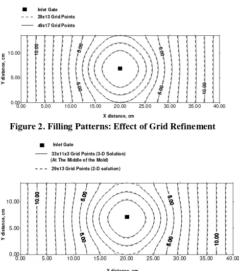
Figure 1 shows that both the 2-D and 3-D models give reasonably good predictions of the experimental data. The calculation with the 2-D program was performed on 49x17 grids, while the 3-D solution was obtained using 33x11x3 grids. Figure 2 shows a comparison of filling patterns obtained from the 2-D model using different grid sizes. It shows that both grid sizes give very similar patterns of filling, i.e. radial flow in the beginning and axial flow in the end. Figure 3 shows a comparison of filling pattern predictions by 2-D and 3-D model using a similar number of grid points. It shows that the models agree with each other very well.
Figure 1. Simulation Results: Non-Reactive System
Figure 2. Filling Patterns: Effect of Grid Refinement
Figure 3. Filling Patterns: Comparison of 2-D and 3-D Model Predictions
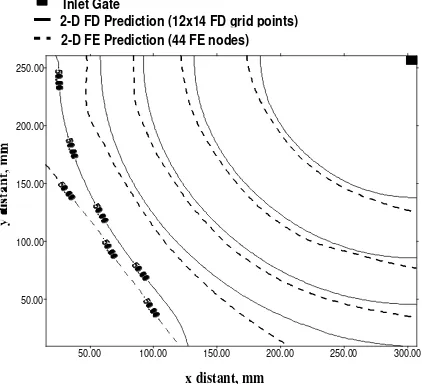
As shown in Figure 4, a comparison was also made with a finite element (FE) based code developed by Dr. Phelan from the United Stated’s National Institute of Standard and Testing (NIST) for a rectangular mold with the dimension of 29.76 cm x 251.5 cm. A 2-D FE mesh was created for a simple rectangular mold with the on Geostar [a platform (both a pre and post-processor) to run FE analysis package Cosmos ; both are the trademarks of Structural Research and Analysis Corporation (SRAC)]. The total number of nodes and elements was 44 and 64, respectively. The mesh information was then translated into a Nastran (one of the most widely used FE code version) format that is readable by Dr. Phelan’s code. Calculations were preformed using both NIST’s FE program and the 2-D version of the FD code. The FD calculation was done on 14x12 grid points. The viscosity of the non-reactive fluid was 100 cp. The preform porosity was 0.8 and its isotropic permeability was 1.85x10⁻⁵ cm2. The gate was located at one of the corners. The fluid injection was assumed to be a constant flow-rate of 10 ml/sec. By using a constant flow rate, the theoretical fill time can be computed since the cavity volume is known. Both codes could predict the theoretical filling time accurately (i. e. 58.7 seconds). The slight difference in front location prediction, as shown in Figure 4, may be caused by the fact that in the FE code the
49x17 Grid Points
0.00 5.00 10.00 15.00 20.00 25.00 30.00 35.00 40.00
0.00 5.00 10.00
29x13 Grid Points Inlet Gate
Y
d
is
ta
n
c
e
,
c
m
X distance, cm
0.00 5.00 10.00 15.00 20.00 25.00 30.00 35.00 40.00
0.00 5.00 10.00
29x13 Grid Points (2-D solution) 33x11x3 Grid Points (3-D Solution) (At The Middle of the Mold)
X distance, cm
Y
d
is
ta
n
c
e
,
c
m
constant flow rate boundary condition is treated as a point source in the corner node, while in the FD code the constant flow rate boundary condition is handled by equally distributing the flow over the area of the inlet gate (the corner control volume).
Figure 4. Comparison with NIST FE Solution: Filling Patterns
All of the simulations show that the FD control volume program gives good predictions for experimental results, as well as some of the FE solutions. Differences in prediction values between the FD solution and the FE solution may be caused by the different ways to store the variables. There is a slight difference in the detailed front locations versus time predicted by FE and FD analysis although both models predict the same overall filling time. This type of difference should diminish as the number of nodes used in the calculation increases.
Conclusion and Recommendation
All simulations, thus far, were performed with non-reacting system. A real test of the developed model is when the simulated process involve reaction and changing rheology such as in reaction injection molding. This should be performed in the future work
References
Cai, Z., and Berdichevsky, A.L., 1993. Numerical Simulation on the Permeability Variations of a Fiber Assembly, Polymer Composites, 14(6), 529-539.
Calhoun, D.R., Yalvac,S., Wetters, D.G., Wu, C.H., Wang, T.J., Tsai, J.S., and Lee, L.J., 1996. Mold Filling Analysis in Resin Transfer Molding, Polym. Comp., 17(2), 251-264.
Cividini, A., and Gioda,G., 1984. An Approximate F.E. Analysis of Seepage with a Free Surface, Int. J. for Num. Analyt. Meth. inGeomechanics, 8, 549-566.
Freitas, C.J., 1995, Perspective: Selected Benchmarks From Commercial CFDS Codes, J. of Fluids Eng., 117.
Friedrichs, B., and Guceri, S.I., 1995. A Hybrid Numerical Technique to Model 3_D Flow Fields in Resin Transfer Molding Processes, Polymer Engineering and Science, 35, 1834-1851.
Gauvin, R., Trochu, F., Lemenn, Y., and Diallo, L., 1996. Permeability Measurement and Flow Simulation Through Fiber Reinforcement, Polym. Comp., 17(1), 34-42.
Hirt, C.W., and Nichols, B.D., 1981. Volume of Fluid (VOF) Method for Dyanamics of Free Boundaries, Journal of Computational Physics, 39, 201-225. Liang, E.W., Wang, H.P., and Perry, E.M., 1993. An
Integrated Approach for Modeling the Injection Compression, and Resin Transfer Molding Processes for Polymer, Advances in Polymer Technology, 12(3), 234-282.
Lin, R.J., Lee, L.J. and Liou, M.J., 1993. Mold Filling and Curing Analysis in Liquid Composite Molding, Polymer Composites, 14(1), 71-81. Lindsay, K.F., 1993. Automation of Preform
Fabrication Makes SRIM Viable for Volume Parts, Modern Plastics, 70(13), 48.
Lo, Y.W., Reible, D.D., Collier, J.R., and Chen, C.H., 1994. 3-Dimensional Modelling of Reaction Injection Molding 2: Application, Polymer Engineering and Science, 34(18), 1401-1405. Macosko, C.W., 1989. RIM: Fundamental of Reaction
Injection Molding, Hanser Publisher, New York. Patankar, S.V., 1980. Numerical Heat Transfer and
Fluid Flow, Hemisphere Publishing Co.
Polushkin, E.Y., Polushkina, O.M., Malkin, A.Y., Kulichikhin, V.G., Michaeli, W., Kleba, I., abd Blaurock, J., 2002. Modeling of structural reaction injection molding. Part II: comparison with experimental data, Polymer Engineering and Science, April.
Rogers, J.K., 1990. RTM and SRIM - ready for main stream Market?, Modern Plastics, 67(12), 44-48. Shojaei, A., Ghaffarian, S.R., and Karimian S.M.H.,
2003. Simulation of the three-dimensional non-isothermal mold filling process in resin transfer molding, Composites Science and Technology, 63, 1931-1948.
Skartis, L., Khomami, B., and Kardos, J.L.,1992, Resin Flow Trough Fiber Beds During Composites Manufacturing Processes, Part II: Numerical and Experimental Studies of Newtonian Flow Through Ideal and Actual Fiber Beds, Polymer Engineering and Science, 32(4), 231-239.
Trochu, F., and Gauvin, R. , 1992. Limitations of a Boundary-Fitted Finite Difference Method for Simulation of the Resin Transfer Molding Process, J. of Reinf. Plastics and Comp., 11(7), 772-786.
50.00 100.00 150.00 200.00 250.00 300.00
50.00 100.00 150.00 200.00 250.00
Inlet Gate
2-D FD Prediction (12x14 FD grid points) 2-D FE Prediction (44 FE nodes)
Trochu, F., Gauvin, R., and Gao, D.M., 1993. Numerical Analysis of the Resin Transfer Molding Process by the Finite Element Method, Advances in Polym. Technology, 12(4), 329-342.
Valenti, M., 1992. Resin Transfer Molding Speed Composite Making, Mechanical Engineering, November.
Wilder, R.V, 1989. Resin Transfer Molding Finally Gets Some Real Attention from Industry, Modern Plastics, July.
Williams, J.G., Morris, C.E.M, and Ennis, B.C., 1074 Liquid Flow Through Aligned Fiber Beds, Polymer Engineering and science, 14(6).
Young, W.B., 1994. Gate Location Optimization in Liquid Composite Molding Using Genetic Algorithms, J. of Comp. Material, 28(12), 1098-1113.
Young, W.B., 1996. The Effect of Surface Tension on Tow Impregnation of Unidirectional Fibrous Preform in Resin Transfer molding, J. of Comp. Materials, 30(11), 1191-1209
Young, W.B., Rupel, K., Han, K., Lee, J.M., and Liou,M.J., 1991. Analysis of Resin Injection Molding in Mold, with Preplaced Fiber Mats, II: Numerical Simulation and Experiments of Mold Filling, Polymer Composites, 12(1), 20-29.