Full Terms & Conditions of access and use can be found at
http://www.tandfonline.com/action/journalInformation?journalCode=ubes20
Download by: [Universitas Maritim Raja Ali Haji] Date: 11 January 2016, At: 19:53
Journal of Business & Economic Statistics
ISSN: 0735-0015 (Print) 1537-2707 (Online) Journal homepage: http://www.tandfonline.com/loi/ubes20
Ambiguity in the Cross-Section of Expected
Returns: An Empirical Assessment
Julian Thimme & Clemens Völkert
To cite this article: Julian Thimme & Clemens Völkert (2015) Ambiguity in the Cross-Section of Expected Returns: An Empirical Assessment, Journal of Business & Economic Statistics, 33:3, 418-429, DOI: 10.1080/07350015.2014.958230
To link to this article: http://dx.doi.org/10.1080/07350015.2014.958230
View supplementary material
Accepted author version posted online: 25 Sep 2014.
Submit your article to this journal
Article views: 151
View related articles
Supplementary materials for this article are available online. Please go tohttp://tandfonline.com/r/JBES
Ambiguity in the Cross-Section of Expected
Returns: An Empirical Assessment
Julian T
HIMMEand Clemens V ¨
OLKERTFinance Center M ¨unster, Westf ¨alische Wilhelms-Universit ¨at M ¨unster, 48149 M ¨unster, Germany ([email protected];[email protected])
This article estimates and tests the smooth ambiguity model of Klibanoff, Marinacci, and Mukerji based on stock market data. We introduce a novel methodology to estimate the conditional expectation, which characterizes the impact of a decision maker’s ambiguity attitude on asset prices. Our point estimates of the ambiguity parameter are between 25 and 60, whereas our risk aversion estimates are considerably lower. The substantial difference indicates that market participants are ambiguity averse. Furthermore, we evaluate if ambiguity aversion helps explaining the cross-section of expected returns. Compared with Epstein and Zin preferences, we find that incorporating ambiguity into the decision model improves the fit to the data while keeping relative risk aversion at more reasonable levels. Supplementary materials for this article are available online.
KEY WORDS: Ambiguity aversion; Asset pricing; Cross-section of returns.
1. INTRODUCTION
Although there is a long tradition to model preferences with subjective expected utility (SEU), researchers nowadays con-sider more sophisticated preference representations. If a deci-sion maker (DM) has vague information about the model that determines the distribution of outcomes, uncertainty does not only appear as risk, that is, fluctuations with a known proba-bility distribution, but also as ambiguity about the model itself. Ambiguity may cause a loss of utility to a DM. The resulting bias in portfolio allocations, mirroring the aspiration for robust de-cision making, might have a perceptible impact on asset prices. This article investigates if ambiguity aversion is present in investors’ decision patterns by looking at the cross-section of stock returns and macroeconomic variables. We estimate a set of preference parameters assuming that investors act in line with the smooth ambiguity (SA) model of preference as devel-oped by Klibanoff, Marinacci, and Mukerji (2005,2009). We compare the model’s pricing performance with the ambiguity-neutral recursive preference model of Epstein and Zin (1989), EZ henceforth, and the pure ambiguity (PA) model that features risk neutrality but ambiguity aversion.
Intuitively, a DM with SA preferences considers a whole set of different economic models. For each, she calculates a cer-tainty equivalent with respect to expected utility. Her decisions are finally based on the expected utility of the set of certainty equivalents with respect to a second utility function. This func-tion displays the DM’s ambiguity attitude and is characterized by the ambiguity parameter η. One goal of this article is to estimate this parameter and thus gauge the ambiguity attitude of investors. An alternative approach to introduce ambiguity aversion is the multiple priors model of Gilboa and Schmeidler (1989). They assumed that a DM does not consider all certainty equivalents belonging to different candidate models, but only the “worst case.” Hansen and Sargent (2001) suggested the re-lation of this approach to the robustness theory of Anderson, Hansen, and Sargent (2000) and Hansen and Sargent (2008). Ju and Miao (2012) pointed out that the SA framework
con-tains these and further preference specifications as special and limiting cases.
Halevy (2007) investigated a variety of decision models using extensions of the Ellsberg (1961) experiment. Bossaerts et al. (2010) and Ahn et al. (2011) analyzed the impact of ambigu-ity in portfolio choice experiments. In contrast to experimental studies, our results are based on historical stock market data. An-derson, Ghysels, and Juergens (2009) and Brenner and Izhakian (2011) also approached empirical evaluations of the impact of ambiguity on asset returns. Both include ambiguity factors that are supposed to capture time-variation in ambiguity about stock returns into linear multi-factor models and find that ambiguity is a priced factor. Similarly, we find evidence for ambiguity in the cross-section of expected returns. As opposed to these ar-ticles, our approach stems from life-cycle consumption-based asset pricing.
Epstein and Schneider (2010) reviewed the literature on am-biguity and asset markets. They concluded that amam-biguity has important implications for the pricing of financial assets. Gen-eral equilibrium asset pricing applications of the SA approach include Collard et al. (2011), Ju and Miao (2012), and Miao, Wei, and Zhou (2012). In these articles, the risk aversion pa-rameterγ is set to a low value, while the ambiguity parame-terηis calibrated to match important asset pricing moments. The assumed values vary significantly between the asset pricing applications in the literature. However, as forγ, there also has to be a reasonable range forη. The findings of Halevy (2007) are interpreted by Chen, Ju, and Miao (in press), who infer an ambiguity parameter between 50 and 90. Our point estimates of ηare between 25 and 60, whileγis clearly lower and within the range considered plausible by Mehra and Prescott (1985). The substantial difference to the risk aversion parameter indicates that market participants are ambiguity averse.
© 2015American Statistical Association Journal of Business & Economic Statistics July 2015, Vol. 33, No. 3 DOI:10.1080/07350015.2014.958230
418
As shown by Mehra and Prescott (1985), the consumption-based asset pricing model of Lucas (1978) and Breeden (1979) has severe problems in explaining the large equity premium and the cross-sectional variation in expected returns. We investigate whether accounting for ambiguity helps explaining these phe-nomena and compare the pricing performances of the SA model with several benchmark models. We find that it is difficult to discriminate between these decision models solely based on pricing errors. The SA model achieves a slightly better fit to the data with low relative risk aversion.
To estimate preference parameters, we use the generalized method of moments (GMM) of Hansen (1982). Hansen and Singleton (1982) employed GMM to estimate the consumption-based capital asset pricing model, while Epstein and Zin (1991) estimated the EZ model. GMM relies on Euler equations to test the fit of candidate pricing kernels. Compared with EZ prefer-ences, the pricing kernel and hence the Euler equation of the SA model contains an additional term, which characterizes the impact of an investor’s ambiguity attitude on asset prices. An ambiguity averse agent puts more weight on economic mod-els that yield a low expected continuation value. Estimation of this expected value, conditional on the economic model, im-poses technical difficulties. Motivated by a long-run risks (LRR) model, we show how to overcome these.
Another difficulty in estimating consumption-based asset pricing models with recursive preferences is that it requires the return on the wealth portfolio, which is not observable. Several approximations have been proposed in the literature. Epstein and Zin (1991) used the return on a broad stock market index. However, Chen, Favilukis, and Ludvigson (2013) and Lustig, Van Nieuwerburgh, and Verdelhan (2012) studied the proper-ties of the return on wealth and found that it is less volatile and only weakly correlated with the return on the stock market. Among others, Campbell (1996) and Jagannathan and Wang (1996) accounted for the large fraction of human wealth in to-tal wealth. As in Zhang (2006), we use a proxy for the return on wealth based on the variablecay of Lettau and Ludvigson (2001), which includes human wealth and total asset holdings.
The remainder of this article is organized as follows. Sec-tion2reviews SA preferences and the pricing kernel. Section
3discusses the estimation technique and its finite sample prop-erties. The preference models are estimated based on post-war consumption and stock market data in Section4. Section5 con-cludes. An online supplementary material provides information about the GMM estimation and a simulation study.
2. SMOOTH AMBIGUITY PREFERENCES
In this section, we briefly review SA preferences. The model’s static version was introduced by Klibanoff, Marinacci, and Muk-erji (2005) and generalized to a dynamic model by Klibanoff, Marinacci, and Mukerji (2009) and Ju and Miao (2012). It is a generalization of recursive preferences as developed by Kreps and Porteus (1978) and Epstein and Zin (1989). Since our goal is to provide a strong intuition for the nature of SA preferences, we set technicalities aside and refer the interested reader to the articles named above.
2.1 The Decision Model
Consider a DM who evaluates future consumption plansC=
(Ct)t∈Nwith respect to the recursive value function
Vt(C)=1−e−δCt1−ρ+e−δ(Rt(Vt+1(C)))1−ρ 1−1ρ
,
where ρ denotes the reciprocal of the DM’s elasticity of in-tertemporal substitution (EIS) andδ the DM’s subjective time discount rate. The uncertainty aggregator Raccounts for risk
and ambiguity in the continuation valueVt+1(C) of future
con-sumption. The aggregation depends on the DM’s attitudes to-ward risk and ambiguity. At each point in timet, the DM faces a model sett. The key assumption of the smooth ambiguity model is that the DM entertains a subjective priorµt, that is, a probability measure ontthat mirrors her assessment of the likelihood of each candidate model intto be the “true” one. A modelis given by a probability measureπt+1∈t on the state space that pins down the distribution of the future consumption stream. We use the subscript t+1 for all models in the time tmodel set to point out that the true model is a random variable int. Each modelπt+1yields a conditional certainty equivalent u−1
Eπt+1[u(Vt+1(C))]
, whereu is a utility function charac-terizing the DM’s risk attitude. The uncertainty aggregator is defined as the unconditional certainty equivalent
Rt(x)=v−1Eµt
vu−1Eπt+1[u(x)]
,
wherevis a further utility function. The ambiguity attitude of the DM depends on the curvature of the compositionφ=v◦u−1.
If it is concave, the DM dislikes mean-preserving spreads in expected utilities conditional on the models int, which implies ambiguity aversion. If it is linear, the DM is ambiguity neutral andRt reduces to the aggregator of EZ preferences.
We assume thatuandvare of the power utility type
u(x)= x erences, whereγdescribes the DM’s attitude toward risk andη her attitude toward ambiguity. She is ambiguity averse ifη > γ. Summing up, at timetthe DM evaluates consumption plansC according to
Equation (1) nests the value functions of EZ preferences (η=
γ) and time-separable constant relative risk aversion (CRRA) utility (ρ=η=γ).
An ambiguity neutral DM does not ignore ambiguity, but is aware of disperse consequences brought forward by different
candidate models in the model sett. However, ambiguity neu-trality means that such a DM aggregates probability distributions corresponding to the candidate models with the help ofµt. The DM thus only considers unconditional probability distributions. To enable a comparison of the preference parameters of an am-biguity averse and an amam-biguity neutral DM, we define the term effective risk aversionas the coefficient of relative risk aversion that yields the same certainty equivalent corresponding to the unconditional probability measure as an ambiguity averse DM that distinguishes between conditional and unconditional prob-ability measures. This definition is motivated by Bonomo et al. (2011), who considered a similar notion for generalized disap-pointment aversion risk preferences, as defined by Routledge and Zin (2010).
The question how the preference parameters of the smooth ambiguity model translate into effective risk aversion depends on the relation between the variance of the conditional distribu-tions (risk) and the variation in certainty equivalents correspond-ing to the conditional distributions (ambiguity). If, for example, the different candidate models yield very similar conditional probability distributions, effective risk aversion is close to the risk aversion coefficientγ as the variance of the unconditional probability measure is largely driven by the variation in the ditional measures. If, however, the variances of all single con-ditional measures are very low, effective risk aversion is biased toward the ambiguity aversion coefficient η. Thus, the defini-tion of effective risk aversion is not canonical but depends on the properties oft and may vary from one decision to the other.
2.2 The Pricing Kernel
The pricing kernelξ links preferences to asset returns via the relation
gross return on money invested at timet for one period in an arbitrary asset i. In complete markets, (ξt,t+1)t∈N is a unique
series of random variables. It can be expressed in terms of continuation values with the help of the value function given in Equation (1). Following Duffie and Skiadas (1994) and Hansen et al. (2007), it satisfies
as reported in Hayashi and Miao (2011), Proposition 8. The first three terms are the EZ pricing kernel, which collapses to the CRRA pricing kernel forγ =ρ. The last term displays the impact of the DM’s ambiguity attitude on asset prices. Its numer-ator is the conditional certainty equivalent of the continuation value as described in Section 2.1. Hence, the DM considers the conditional certainty equivalent corresponding to a certain economic model πt+1 relative to the unconditional certainty
equivalent. Depending on her ambiguity attitude, she puts more (if ambiguity averse, that is,γ < η) or less (if ambiguity
lov-ing, i.e.,γ > η) weight on economic models that yield a low expected utility.
The continuation value is unobservable and in applications it is usually more convenient to work with the pricing kernel in terms of the return on wealth. We defineθ1:= 11−−γρ andθ2 :=
where Rw denotes the return on the wealth portfolio, that is, the claim on aggregate consumption. The parameter θ2
ex-presses the concavity ofφand therefore the ambiguity attitude of the DM. Hence, the bias through the additional last term in the pricing kernel (compared to the EZ pricing kernel) causes the impact of the DM’s ambiguity attitude on asset prices.
We decompose the pricing kernel into three parts ξt,t+1= ξCRRA
and consider a number of special cases. Assuming γ =η yields the ambiguity neutral Epstein–Zin pricing kernel, as ξSA equals 1. Likewise, if ρ=γ, then ξEZ equals 1 and ξt,t+1=ξt,tCRRA+1 ×ξ
SA
t,t+1. We refer to this case as pure ambi-guity(PA) preferences. This term is justifiable as the impact of ξCRRA is negligible in our applications. A pure ambiguity in-vestor cares for covariation of model-implied expected returns with model-implied expectations of consumption growth and return on wealth. Consider the assumptionρ=γ =0, which further facilitates the pricing kernel asξCRRA trivializes to the
constant time discount ratee−δ. Equation (2) is then given by
In this section, we introduce the econometric methodology to infer attitudes toward ambiguity from financial market data. We use GMM to estimate the preference parameters. From Equa-tion (4), it is clear that two central components of the pricing kernel are the return on the wealth portfolio, which cannot be observed at the market, and the expected value, conditional on the economic model, that distinguishes SA from EZ prefer-ences. We discuss a return proxy in Section3.2and provide an estimation technique for the conditional expectation in Section
3.3. Section 3.4summarizes the results of a simulation study that investigates the finite sample properties of our estimation technique. Details on the simulation study can be found in the online supplementary material.
3.1 GMM Estimation
Euler equations link asset returns to consumption growth and the return on the wealth portfolio. The imposed population mo-ment restrictions can be employed to test the fit of candidate pricing kernels. To weight the moment conditions, we use the identity matrix. Minimizing the sum of squared pricing errors makes the results comparable to asset pricing tests using ordi-nary least-square (OLS) cross-sectional regressions. In addition, the identity matrix is suitable for comparing SA preferences with the benchmarks of EZ and PA preferences, as it is invariant across all models tested. According to Altonji and Segal (1996), first-stage GMM estimates are also more robust in finite sam-ples. Cochrane (2005, chap. 11) explained several additional advantages of using a prespecified weighting matrix.
The null hypothesis that all moment conditions are zero can be tested using Hansen’sJ-test. If we acknowledge that all models are misspecified, hypotheses tests of the null of correct model specification against the alternative of incorrect specification are of limited value. Following the idea that we are looking for the least misspecified model, we compare root mean squared errors (RMSE) and Hansen and Jagannathan (1997) distances (HJD) of different preference specifications and parameter vectors. We test if these performance measures are zero using the methodol-ogy proposed by Jagannathan and Wang (1996) and Parker and Julliard (2005). We use a Wald test to evaluate the restriction ρ=γ, which corresponds to time separability in the EZ model and to pure ambiguity preferences in the SA model. We further-more evaluate the restriction for ambiguity neutrality (γ =η). Details on the estimation procedure and on testing hypotheses are provided in the online supplementary material.
Ferson and Foerster (1994), Hansen, Heaton, and Yaron (1996), Smith (1999), and Ahn and Gadarowski (2004) pointed out that commonly employed specification tests reject too often in finite samples. Thus, relying solely on these tests to evaluate the goodness of fit of candidate asset pricing models is problem-atic. Lewellen, Nagel, and Shanken (2010) showed that focusing too closely on high cross-sectionalR2’s and small pricing errors
can be misleading and that it is important to evaluate if the deci-sion models produce plausible preference parameter estimates. Allowing all parameters to be estimated freely focuses solely on model fit. Restricting certain preference parameters to eco-nomically reasonable values, balances the objective between minimizing pricing errors and the plausibility of the parameter estimates. We follow Bansal, Gallant, and Tauchen (2007) and fix the EIS at economically reasonable values. There is consid-erable debate about the correct value of the EIS. Hall (1988), Campbell and Mankiw (1989), and Yogo (2004) found an EIS close to zero, while Vissing-Jørgensen and Attanasio (2003), Bansal and Yaron (2004), Guvenen (2006), and Chen, Fav-ilukis, and Ludvigson (2013) argued for a higher value. Hansen, Heaton, and Li (2008) and Malloy, Moskowitz, and Vissing-Jørgensen (2009) set the EIS to one. This choice simplifies the analysis considerably. However, it implies that the
wealth-consumption ratio is constant. Lettau and Ludvigson (2001) and Lustig, Van Nieuwerburgh, and Verdelhan (2012) showed that this contradicts empirical evidence. In the LRR model of Bansal and Yaron (2004), a drop in volatility and a rise in expected consumption growth increase the wealth-consumption ratio if the EIS is greater than one. Bansal, Khatchatrian, and Yaron (2005) supported the negative relation between volatility and as-set prices and Lustig, Van Nieuwerburgh, and Verdelhan (2012) showed that the LRR model produces a wealth-consumption ratio that fits the data.
As suggested by Constantinides and Ghosh (2011), we report results for several values of the EIS. Prefixing the EIS is benefi-cial for several reasons. First, it is very difficult to estimate the EIS reliably. As our main object of interest is the DM’s attitude toward ambiguity and not the magnitude of the EIS, setting it to economically reasonable values simplifies the estimation of the ambiguity parameter. Second, it facilitates the comparison of parameter estimates of the EZ and SA models, that is, the ef-fect that differences in the estimated EIS cause large changes in the estimated values of risk and ambiguity aversion is avoided. Furthermore, fixing the EIS at reasonable levels may provide valuable guidance on the magnitude of risk and ambiguity aver-sion for researchers in calibrating the SA model.
3.2 Return on Wealth
Testing candidate pricing kernels corresponding to recursive preference models presumes that either the continuation value of the future consumption plan in Equation (3) or the return on the wealth portfolio in Equation (4) is observable. The wealth portfolio is an asset that pays aggregate consumption as divi-dends. Although aggregate consumption is observable, neither the return on aggregate wealth nor the continuation value can be observed at the market. This causes severe problems for estimat-ing consumption-based asset pricestimat-ing models, as pointed out by Ludvigson (2012). Approximating the continuation value is dis-cussed in Hansen, Heaton, and Li (2008), Ju and Miao (2012), and Chen, Favilukis, and Ludvigson (2013).
Approximating the return on wealth with a suitable func-tion of observable variables is another alternative. Epstein and Zin (1991) approximated the return on aggregate wealth by the return on a broad stock market index. Among others, Stock and Wright (2000) and Yogo (2006) followed this approach. However, a stock market index is only a good approximation to the return on aggregate wealth if human capital and other nontradable assets are minor components of aggregate wealth. Critique of this approach goes back to Roll (1977). Lustig, Van Nieuwerburgh, and Verdelhan (2012) showed that human cap-ital makes up the largest fraction of aggregate wealth. Camp-bell (1996) and Jagannathan and Wang (1996) included hu-man capital. However, other components of wealth, such as total household asset holdings, should also be accounted for. We discuss an approach that incorporates all kinds of wealth by using the cay variable, defined by Lettau and Ludvigson (2001).
cayapproximates innovations in the log consumption-wealth ratio. The authors assumed that asset holdings and human capital sum up to total wealth and that human wealth is approximately
proportional to labor income.cayis defined as
cayt :=ct−ωat−(1−ω)yt,
where c denotes log consumption, a log asset holdings, and ylog aggregate labor income. The Appendix contains precise specifications of the variables used. The variableωis the relative share of asset holdings in total wealth, which is assumed to be constant over time. Lettau and Ludvigson (2001) proposed that c,a, andyare cointegrated and estimate the coefficientsωand 1−ωusing OLS. Since the estimates do not perfectly sum up to 1, we proceed as Zhang (2006) and divide the estimate ofω by the sum of both estimates.
Let Wt denote aggregate wealth at time t. Using the bud-get constraintWt+1=(Wt−Ct)Rwt,t+1, the return on wealth is
Labor income does not enter the budget constraint explicitly, but implicitly through the assumption that human capital is a part of aggregate wealth. We assume that Ct
Wt =κ·exp(cayt), that is,
the consumption-wealth ratio fluctuates around its steady state valueκ. An approximation to the return on wealth is
Rt,tcay+1:=Ct+1
Ct
exp(cayt−cayt+1)
1−κ·exp(cayt) .
We setκ in line with the values given in Lettau and Ludvigson (2001), which yields an average consumption-wealth ratio of about 1/25 in annual terms. The constantκis of minor relevance for the estimation, since it is the timing of innovations to the consumption-wealth ratio rather than its level that is important for the estimation. Setting the average ratio to 1/83, as reported by Lustig, Van Nieuwerburgh, and Verdelhan (2012), yields parameter estimates that are virtually the same.
Table S1 in the online supplementary material contains sum-mary statistics of the proxyrcay =logRcay. Its mean is about 1.5% per quarter and thus slightly lower than the average stock market return. Moreover,rcayhas similar statistical properties as the return on wealth in Chen, Favilukis, and Ludvigson (2013). They found that the return on aggregate wealth is less volatile compared with the return on the Center for Research in Security Prices (CRSP) stock market index and the correlation between the two is rather low. In our sample, the standard deviation is less than one tenth of the standard deviation of the CRSP stock market index and the correlation between the two return series is 0.51.
3.3 Estimation of the Conditional Expectation
Using Euler equations to estimate the SA model requires an empirical estimate of the conditional expectationEπt+1[Yt+1],
We assume that the conditional expectation ofYt+1is a function
of a standardized vectorXt+1of timet+1 regressors. For the
approach to be valid, the economic model needs to be explicable
by these regressors. More precisely, there has to be a bijective relation between the set of economic modelsand the image ofX, that is, all possible realizations of the regressor variables. Which variables are suited to identify the economic model? The risk-free rate and the log price-dividend ratio are observable, show a clear business cycle pattern, and have a long tradition as predictors of stock and bond returns. Cochrane (2005, chap. 20) provided a detailed review of the literature. Furthermore, in standard affine asset pricing models, as, for example, those of Bansal and Yaron (2004) and Drechsler and Yaron (2011), these variables are approximately affine in the state vector that pins down the distribution of consumption and dividend growth. Among others, Constantinides and Ghosh (2011) and Bansal, Kiku, and Yaron (2012) exploited this relation to estimate LRR models. In the models they considered, these two variables span the state space. This also holds if the representative investor is ambiguous about the distribution of consumption and dividend growth. They inverted the expressions for the log price-dividend ratio and the risk-free rate to express the state variables in terms of observables. Because of their economic relevance and moti-vated by the relation in affine asset pricing models, we use these two quantities and their first lags as predictor variables.
We run a locally linear regression
log(Yt+1)=m(Xt+1)+(Xt+1)εt+1, t ∈ {0, . . . , T −1},
whereis the conditional volatility andεdenotes an iid zero mean, unit variance disturbance term, and interpret the fitted valuem(Xt+1) as the conditional expectation. Using logs
cor-responds to minimizing the squared relative error that is rea-sonable, since the conditional expectation is multiplied by other terms in the Euler equations. Moreover, it guarantees that the predictedYt+1as a part of the SA pricing kernel is positive. We
allow for nonlinearities inmand approximate the conditional expectation locally by a linear function. Nagel and Singleton (2011) used a similar approach to estimate conditional mo-ments. Fan (1992) and Ruppert and Wand (1994) showed that the local linear estimator has several advantages compared to other nonparametric estimators. For eachi∈ {0, . . . , T −1}, an estimate of the conditional expectation at the data pointXi+1
is
The weighting functionwassigns more weight to observations close to the current data point and less weight to observations farther away. Ifldenotes the number of explanatory variables, that is, the length of the vectorXt+1for anyt ∈ {0, . . . , T −1},
the weighting function is defined as
w(X1, X2) :=
The weighting depends on the specification of the kernel func-tionK, which assigns local weights to the linear estimator. The
vector of bandwidthsh=(h1, . . . , hl) controls the
neighbor-hood of the current point. As Nagel and Singleton (2011), we use the Epanechnikov kernelK(u)= 34(1−u2)1
(|u|≤1), which
minimizes the mean squared deviation of the corresponding kernel density estimator. We also employ other kernel functions (not reported) and find that the choice of the kernel does not alter the results. We allow for an individual bandwidth for each regressor. A large bandwidthhiresults in a smooth estimate that might neglect important features of the data contained in theith regressor, while for a small bandwidth the estimate follows the data very closely. The optimal vector of bandwidthshis chosen by minimizing the cross-validation criterion
CV(h)= 1
T T−1
i=0
log(Yi+1)−( ˆαi−+1+βˆ
− i+1Xi+1)
2 ,
where [ ˆαi−+1,βˆi−+1] denotes the estimate computed excluding the (i+1)th data point. In our applications, the bandwidths range from 2.8 to 6.6. They are larger for the contemporaneous regressors than for the first lags and increase inρ.
3.4 A Simulation Study
We estimate the SA model based on simulated consumption and return data to investigate the performance of our estima-tion technique in finite samples. To simulate data, we rely on a long run risks model similar to that of Bansal and Yaron (2004), in which the distribution of consumption and divi-dend growth depends on two state variables: Trend consumption growth and economic uncertainty. Both are modeled as mean-reverting processes. We assume that the representative investor perceives innovations in the state variables as ambiguous. We simulate return data given that the investor is ambiguity averse with SA =(ρ=0.667, δ=0.0033, γ =5, η=20) and use
the parameterization of Bansal, Kiku, and Yaron (2012) for all other parameters. As discussed in Section3.1, we fixρat 0.667 and estimate the remaining preference parameters. Details on the model and its solution, as well as an extensive discussion of the results of the simulation study can be found in the online supplementary material.
We find that the point estimates of the preference parameters are very close to the imposed values, however, with large stan-dard errors forηand especiallyγ. This indicates that it is rather difficult to estimate the risk aversion and ambiguity parameters jointly in small samples. The large standard error of the risk aversion coefficient implies that ambiguity neutrality (γ =η) is difficult to reject. Even though the model is true, the median p-value of the Wald test is above 10%. We also run simulations with larger samples (100, 200, 500, and 1000 years). The Wald tests reject ambiguity neutrality for sample sizes of 100 years and above.
In addition, we investigate the bias if the parameters are esti-mated assuming EZ or PA preferences but the data were gener-ated given the SA model. In case of EZ preferences, the median risk aversion estimate is 14.29, which can be interpreted as the effective risk aversion of the ambiguity averse investor with
SA. It is clearly above the assumed risk aversion coefficient of
5. Thep-values of the specification test based on the HJD and theJ-test are slightly below 5%. The RMSE is close to the one
given the full model is estimated. These results show that even if ambiguity aversion is present, it is rather difficult to discrim-inate between SA and EZ models solely based on their pricing errors in small samples. The same is true for the PA model, which is not rejected by any of the specification tests although it is misspecified.
Concerning the finite sample properties of the specification tests, we are able to draw several conclusions. We observe that in our simulation study, the rejection rates are far too large for samples smaller than 500 years. This confirms that the test rejects too often for sample sizes typically used in empirical tests of consumption-based asset pricing models. Similar to Ahn and Gadarowski (2004), we find that the specification test based on the Hansen and Jagannathan (1997) distance also performs poorly in small samples. In line with Parker and Julliard (2005), we find that the test based on the RMSE behaves superior in finite samples.
4. EMPIRICAL EVIDENCE
In this section, we estimate the preference parameters based on consumption and stock market data. Furthermore, we ana-lyze the evolution of the estimated pricing kernels and investi-gate the in-sample and out-of-sample pricing performances of the alternative preference models. The sample period is from the first quarter of 1952 to the third quarter of 2011.Rcayis used as proxy for the return on wealth. The set of test assets includes the 3-month Treasury bill, the CRSP value weighted stock market index, 10 portfolios formed on size, 10 book-to-market value sorted portfolios, and 10 industry portfolios. We use alternative sets of test assets to explore the sensitivity of the results in Sec-tion4.2. The data are described in the Appendix. Table S1 in the online supplementary material contains descriptive statistics of the variables used in the estimation.
4.1 Parameter Estimates
The estimated parameters and their standard errors are shown inTable 1. All results are reported for two values of the EIS, 1.5 and 2. These values are typically used in asset pricing studies with recursive preferences. As outlined in Section3.1, restrict-ing the value of ρ has several advantages. To verify that the assumed values are in line with empirical evidence, we esti-mate the models treatingρas a free parameter. We obtain point estimates close to the values above (not reported). However, standard errors are very large, as the objective function is very flat inρ. The problem of getting precise estimates of the EIS has also been reported by Bansal, Gallant, and Tauchen (2007) and Constantinides and Ghosh (2011), among others. Moreover, we study the caseρ=0,which is interesting from a theoretical point of view asγ =ρyields risk neutrality.
For the SA model, the estimated vectors ˆSA are (0.000,0.014,7.016,61.035), (0.500,0.012,2.295,35.091), and (0.667,0.011,0.819,24.817). The subjective time discount rate is approximately 5% per annum and estimated with great precision. The risk aversion coefficients are estimated within the range considered plausible by Mehra and Prescott (1985), however, with large standard errors. The point estimates of the ambiguity parameter η are considerably larger than the
Table 1. Parameter estimates
ρ δ γ η R2 RMSE HJD γ=ρ η=γ J-test
Panel 1: SA (ρrestricted)
0.000 0.014 7.016 61.035 0.483 0.020 0.620 0.027 1.170 90.804 (–) (0.000) (42.873) (21.034) (–) (0.090) (0.000) (0.870) (0.279) (0.000) 0.500 0.012 2.295 35.091 0.477 0.020 0.612 0.004 1.125 85.991 (–) (0.000) (26.836) (11.744) (–) (0.088) (0.000) (0.947) (0.289) (0.000) 0.667 0.011 0.819 24.817 0.474 0.020 0.608 0.000 1.184 84.046 (–) (0.000) (19.217) (8.146) (–) (0.084) (0.000) (0.994) (0.276) (0.000)
Panel 2: EZ (ρrestricted)
0.000 0.013 55.104 0.383 0.021 0.696 7.579 86.299
(–) (0.001) (20.016) (–) (0.253) (0.000) (0.006) (0.000)
0.500 0.011 31.075 0.403 0.021 0.690 8.130 91.679
(–) (0.001) (10.723) (–) (0.239) (0.000) (0.004) (0.000)
0.667 0.010 21.843 0.402 0.021 0.690 8.211 92.921
(–) (0.001) (7.390) (–) (0.233) (0.000) (0.004) (0.000)
Panel 3: PA (ρ=γrestricted)
0.000 0.014 0.000 61.960 0.481 0.020 0.614 8.618 93.827
(–) (0.000) (–) (21.106) (–) (0.136) (0.000) (0.003) (0.000)
0.500 0.012 0.500 35.302 0.477 0.020 0.609 8.880 93.441
(–) (0.000) (–) (11.679) (–) (0.122) (0.000) (0.003) (0.000)
0.667 0.011 0.667 24.833 0.474 0.020 0.608 8.944 93.447
(–) (0.000) (–) (8.081) (–) (0.116) (0.000) (0.003) (0.000)
NOTE: The table shows GMM estimates of the preference parameters. SA refers to the smooth ambiguity model, EZ to Epstein and Zin (1989) preferences, and PA to pure ambiguity preferences. HAC standard errors are in parentheses. The RMSE is the square root of the mean squared Euler equation error. HJD denotes the Hansen and Jagannathan (1997) distance. The table also reports the cross-sectionalR2, the Wald tests for the hypothesesγ=ρandη=γ, and theJ-test for overidentifying restrictions (p-values in parentheses). Details on the tests are provided in the online supplementary material.
risk aversion estimates. As in our simulation study, the large standard errors of the risk aversion and ambiguity parameters show that these parameters are hard to estimate precisely. An economic interpretation why it is difficult to identify the two parameters separately is that once the agent knows the economic model, the remaining uncertainty of the distribution of returns might be of minor relevance. If returns are well described by the economic model, ambiguity accounts for a major part of the overall uncertainty and the impact of risk aversion on asset prices is relatively small.
The ambiguity parameter increases in the value of the EIS. For the intuition of this result, consider the long-run risks model with ambiguity about the state variables, in which the market prices of the long-run risk factors are proportional toθ1θ2−1 (see the
structural equations provided in the online supplementary ma-terial). When estimating the preference parameters, returns are given exogenously. Consequently, the representative investor’s preferences just influence the pricing kernel and thus the mar-ket prices of risk. To match the equity premium in the data, an increase in ρ is compensated by a lower value of η, as long as ρ <1. SA preferences price the cross-section of expected returns rather well and an RMSE of zero cannot be rejected. The other two specification tests, theJ-test and the test based on the HJD, reject the model. However, we have seen in Section
3.4that the finite sample properties of these two tests are rather poor.
Assuming EZ preferences, that is, estimating the param-eters given η=γ, yields ˆEZ of (0.000,0.013,55.104), (0.500,0.011,31.075), and (0.667,0.011,21.843). The point estimates of relative risk aversion are clearly above the values considered plausible by Mehra and Prescott (1985). This
indi-cates that these estimates may correspond to the effective risk aversion of investors and that we estimate a misspecified model, which counterfactually neglects ambiguity and the investor’s ambiguity aversion. Malloy, Moskowitz, and Vissing-Jørgensen (2009) argued that the EIS has little impact on the risk aversion estimate if the estimation is solely based on the cross-sectional variation in returns. In contrast to their study, we force the mod-els to also match the equity premium. We observe that higher values of the EIS lead to larger estimates of the risk aversion parameter. As above, this may be explained by the standard long-run risks model, in which the market prices of long-run risks are proportional toθ1−1.
Estimating preference parameters under the assumption of PA preferences, that is, imposingρ=γ, yields point estimates of δandηthat are similar to those if SA preferences are estimated. The pricing performance with respect to cross-sectionalR2and RMSE is equal to that of the SA model. This was expected, as the hypothesisρ=γis far from being rejected in the SA model due to low point estimates in combination with large standard errors ofγ. Note thatρ=γ does not imply time separability in case of SA and PA preferences asηis significantly different fromρ. Time separability is rejected in all three models.
We find the relation ˆγSA<γˆEZ<ηˆSA<ηˆPA. In light of the
results of our simulation study, ˆγEZ might be interpreted as
the effective risk aversion of ambiguity averse investors. The result that the ambiguity parameter is estimated above the risk aversion coefficient indicates the presence of ambiguity aversion in the cross-section of expected returns. The null hypothesis of ambiguity neutrality is not rejected by the Wald test. However, this has to be put into perspective to the finite sample evidence in the simulation study (see the online supplementary material),
where the Wald test did not reject ambiguity neutrality even in the presence of ambiguity aversion.
4.2 Sensitivity of the Parameter Estimates
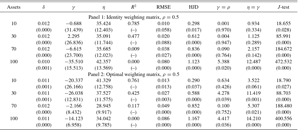
To explore the sensitivity of the results with respect to the number of test assets, we also estimate the SA model using 10, 70, and 100 portfolios in addition to the 3-month Treasury bill and the return on the CRSP stock market index. The 10 portfolios contain 5 size-sorted and 5 value-sorted portfolios, while the 70 portfolios contain 10 size-sorted, 10 value-sorted, 30 industry-sorted portfolios, 10 portfolios industry-sorted by long-term reversal, and 10 sorted by dividend yield. The 100 portfolios are double-sorted by size and book-to-market value. Estimation results are given in Panel 1 ofTable 2. Details about the portfolios can be found in the Appendix.
For all estimations, we fix the EIS at 2. The point estimates of all parameters are not statistically different for the different sets of test portfolios. Point estimates of the ambiguity parameter range from 35 to 42. If 100 portfolios are used in the estimation, the Wald test rejects ambiguity neutrality. In this case, the esti-mated risk aversion coefficient is negative. Negative estimates ofγare also reported by other studies, for example, Hansen and Singleton (1996) and Parker and Julliard (2005). Neely, Roy, and Whiteman (2001) noted that point estimates ofγ are quite sensitive to the choice of test assets.
We also report parameter estimates using the optimal weight-ing matrix in Panel 2 of Table 2. The point estimates of all three parameters are in line with the estimates reported in Panel 1. Especially, the estimates of the ambiguity parameter ηare fairly robust and range from 29 to 41. The RMSEs are larger, indicating that the optimal weighting matrix puts less emphasis on accurately pricing the original test assets. Due to the greater
precision of the parameter estimates, ambiguity neutrality is re-jected. This result supports our main finding that investors are ambiguity averse and that this attitude affects assets returns.
4.3 Estimated Pricing Kernel
The upper panel of Figure 1 shows the pricing kernels of the three decision models, given ˆSA=
(0.500,0.012,2.295,35.091), ˆEZ=(0.500,0.011,31.075), and ˆPA =(0.500,0.012,0.500,35.302), that is, point esti-mates reported inTable 1. The shaded areas represent NBER recessions. The estimated pricing kernels are always positive and thus satisfy the no arbitrage condition. Economic theory suggests that an investor evaluates payoffs more highly when economic conditions are bad, that is, during recessions.Figure 1
shows that the realized pricing kernels have a clear business cy-cle pattern. As consumption growth and the return on wealth are low during recessions, the realized pricing kernels are highest during these periods.
The realized pricing kernels show a similar behavior over time. In the estimation, we force the mean of the realized pricing kernel to match the inverse of the average real quarterly gross return on the risk-free asset, which is 1.0029 in our sample. Thus, the average pricing kernels are all close to one.Figure 1
shows that the peaks in the pricing kernel are more pronounced for the EZ model. Especially during the recent financial crisis the pricing kernel of the EZ model reached a value of 5.14 in contrast to only 1.82 for the PA model. An ambiguity averse investor pays relatively little attention to single extreme outcomes in consumption growth and the return on wealth. She rather cares about the expected utility conditional on the economic model at hand, respectively, its certainty equivalent, which leads to less extreme values of the pricing kernel.
Table 2. Sensitivity of parameter estimates
Assets δ γ η R2 RMSE HJD γ =ρ η=γ J-test
Panel 1: Identity weighting matrix,ρ=0.5
10 0.012 −0.688 35.424 0.785 0.010 0.298 0.001 0.934 18.655 (0.000) (31.439) (12.403) (–) (0.058) (0.017) (0.970) (0.334) (0.028) 30 0.012 2.295 35.091 0.477 0.020 0.612 0.004 1.125 85.991 (0.000) (26.836) (11.744) (–) (0.088) (0.000) (0.947) (0.289) (0.000) 70 0.012 −6.615 35.685 0.009 0.038 0.836 0.090 2.157 184.672 (0.000) (23.700) (12.023) (–) (0.027) (0.000) (0.764) (0.142) (0.000) 100 0.010 −35.510 42.357 0.000 0.080 1.123 5.388 12.487 472.532 (0.001) (15.513) (13.569) (–) (0.000) (0.000) (0.020) (0.000) (0.000)
Panel 2: Optimal weighting matrix,ρ=0.5
10 0.011 −20.337 41.329 0.761 0.013 0.290 0.634 3.522 18.790 (0.001) (26.166) (12.758) (–) (0.013) (0.037) (0.426) (0.061) (0.027) 30 0.011 −26.038 37.527 0.425 0.027 0.588 4.278 11.419 88.703 (0.001) (12.831) (11.575) (–) (0.003) (0.000) (0.039) (0.001) (0.000) 70 0.012 −2.166 28.945 0.117 0.049 0.852 0.100 5.307 188.480 (0.000) (8.432) (9.917) (–) (0.000) (0.000) (0.752) (0.021) (0.000) 100 0.011 −14.123 34.042 0.000 0.086 1.167 4.417 14.210 400.556 (0.000) (6.958) (9.785) (–) (0.000) (0.000) (0.036) (0.000) (0.000)
NOTE: The table shows GMM estimates of the preference parameters of the smooth ambiguity model with varying sets of test assets. The different sets of test assets are described in the Appendix. Panel 1 shows results given the identity matrix is used for weighting the moment conditions, Panel 2 shows results if the optimal weighting matrix is used. HAC standard errors are in parentheses. The RMSE is the square root of the mean squared Euler equation error. HJD denotes the Hansen and Jagannathan (1997) distance. The table also reports the cross-sectionalR2, the Wald tests for the hypothesesγ=ρandη=γ, and theJ-test for overidentifying restrictions (p-values in parentheses). Details on the tests are provided in the online supplementary material.
19500 1960 1970 1980 1990 2000 2010 1
2 3 4 5
ξ
SA EZ PA
1950 1960 1970 1980 1990 2000 2010
−4 −2 0 2 4 6
ξ
(Standardized)
ξCRRA ξEZ ξSA
Figure 1. Realized pricing kernels. The figure shows time-series of realized pricing kernels for the three decision models in the upper panel. It also displays the standardized components of the decomposition in Equation (5) in the lower panel. SA refers to smooth ambiguity preferences, EZ to Epstein and Zin (1989) preferences, PA to pure ambiguity preferences. The EIS is set to 2. The shaded areas represent NBER recessions.
To provide deeper insights into how ambiguity distorts the pricing kernel, we consider the pricing kernel decomposition in Equation (5). If investors know the economic model, the conditional expectation is a constant and does not contain any additional information. If ambiguity is present and investors care about it, the question is whether the conditional expecta-tion matters for the pricing of assets. To improve the fit to the cross-section of expected returns, ξSA has to carry additional
information compared withξCRRA andξEZ. The sample
corre-lation between ξCRRA andξSA is about 0.25. If ξEZ and ξSA
have a correlation close to one, the introduction of ambiguity is basically relabeling risk as ambiguity. For the realized pricing kernel of the SA model, the sample correlation betweenξEZand ξSAis 0.53. This shows that ambiguity matters for asset prices.
4.4 Pricing Performance
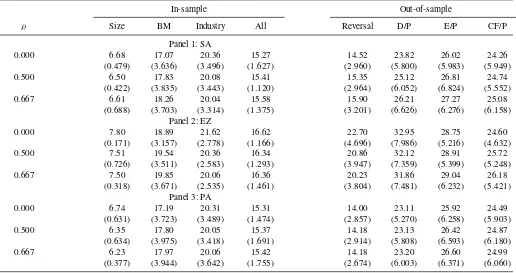
Table 3reports cross-sectional relative pricing errors (in per-cent), which are the square roots of the mean squared differ-ences between realized and predicted returns divided by the square roots of the mean squared returns. We use the sample covariance between the pricing kernel and the portfolio returns to calculate predicted returns (details are provided in the online supplementary material).
How can ambiguity help explaining the equity premium and the cross-sectional variation in expected returns? The EZ model only accounts for the covariation of returns with consumption growth and the return on wealth. The pricing kernel of the SA model contains the additional termξSA. Hence, it also accounts
for the covariance between returns and the continuation value of the timet+1 economic model. The PA model accounts ex-clusively for the latter. Consider a portfolio that has low returns whenever the economic model is unfavorable, that is, when it yields a low continuation value. Ambiguity averse investors command a premium for bearing this uncertainty (ambiguity premium). Compared to the EZ model, the expected return on such an asset is higher given SA preferences. Thus, the SA
model may help explaining the returns of portfolios, which are highly exposed toξSA. If consumption growth and the return on wealth already characterize the economic model rather well, that is,ξCRRA×ξEZ andξSA are highly correlated, the ambi-guity premium can be replicated by amplifying the risk factors of the EZ model. This can be achieved by using a high value of relative risk aversion. In Section4.3, we have seen that the correlation is 0.53. Thus, we expect the risk factors of the EZ model to replicate the ones of the SA model to some extent, but not entirely.
Both models perform similarly in matching the equity pre-mium. In the data, it is 1.61% per quarter, while it amounts to 2.01% in the SA model, 2.05% in the EZ model, and 1.94% in the PA model. To quantify the contribution of ambiguity in the SA model, we decompose the model-implied equity premium into a risk premium and an ambiguity premium by using the log linear approximation
−cov(ξ
CRRAξEZξSA,
R)
E[ξ] ≈ −
cov(ξCRRAξEZ,R)
E[ξ] −
cov(ξSA,R)
E[ξ] .
Given ρ=0.5, we find that the risk premium accounts for 31.19% of the equity premium, while the ambiguity premium makes up the remaining 68.81%.
Table 3shows that it is difficult to discriminate between the models based on their pricing performances. All models have difficulties in accurately pricing book-to-market and industry portfolios. The pricing errors of the 10 size sorted portfolios are considerably lower, with the ambiguity sensitive models slightly outperforming. Concerning the industry sorted portfo-lios, although the average pricing performance is similar across models, there are some noteworthy differences for the individ-ual industries. The absolute pricing error of industry portfolio 1 (nondurables) reduces from 0.76% in the EZ model to 0.43% in the PA model, while for industry portfolio 4 (energy) it in-creases from 0.20% to 0.54%. Consistent with the arguments above, the correlation between the return on portfolio 1 andξSA
is relatively large in absolute terms, while it is low for portfolio
Table 3. Pricing errors
In-sample Out-of-sample
ρ Size BM Industry All Reversal D/P E/P CF/P
Panel 1: SA
0.000 6.68 17.07 20.36 15.27 14.52 23.82 26.02 24.26
(0.479) (3.636) (3.496) (1.627) (2.960) (5.800) (5.983) (5.949)
0.500 6.50 17.83 20.08 15.41 15.35 25.12 26.81 24.74
(0.422) (3.835) (3.443) (1.120) (2.964) (6.052) (6.824) (5.552)
0.667 6.61 18.26 20.04 15.58 15.90 26.21 27.27 25.08
(0.688) (3.703) (3.314) (1.375) (3.201) (6.626) (6.276) (6.158) Panel 2: EZ
0.000 7.80 18.89 21.62 16.62 22.70 32.95 28.75 24.60
(0.171) (3.157) (2.778) (1.166) (4.696) (7.986) (5.216) (4.632)
0.500 7.51 19.54 20.36 16.34 20.86 32.12 28.91 25.72
(0.726) (3.511) (2.583) (1.293) (3.947) (7.359) (5.399) (5.248)
0.667 7.50 19.85 20.06 16.36 20.23 31.86 29.04 26.18
(0.318) (3.671) (2.535) (1.461) (3.804) (7.481) (6.232) (5.421) Panel 3: PA
0.000 6.74 17.19 20.31 15.31 14.00 23.11 25.92 24.49
(0.631) (3.723) (3.489) (1.474) (2.857) (5.270) (6.258) (5.903)
0.500 6.35 17.80 20.05 15.37 14.18 23.13 26.42 24.87
(0.634) (3.975) (3.418) (1.691) (2.914) (5.808) (6.593) (6.180)
0.667 6.23 17.97 20.06 15.42 14.18 23.20 26.60 24.99
(0.377) (3.944) (3.642) (1.755) (2.674) (6.003) (6.371) (6.060)
NOTE: The table reports relative cross-sectional pricing errors (in percent), which are computed by taking the square roots of the mean squared differences between realized and predicted returns divided by the square roots of the mean squared returns. The standard errors in parentheses are calculated by bootstrapping using 10,000 replications. SA refers to the smooth ambiguity model, EZ to Epstein and Zin (1989) preferences, and PA to pure ambiguity preferences. The construction of predicted returns is described in Section S1 of the online supplementary material. To evaluate the in-sample pricing performance of the models, we rely on 10 size sorted, 10 value sorted, and 10 industry portfolios. “All” contains 10 size, 10 book-to-market, and 10 industry sorted portfolios. These portfolios, together with returns on a Treasury bill and CRSP value weighted stock index are used to estimate the parameters. To evaluate the out-of-sample pricing performance, we look at 10 portfolios formed on long-term reversal, 10 dividend yield sorted portfolios, 10 portfolios formed on earnings to price ratios, and 10 cash-flow to price sorted portfolios. The construction of the individual portfolios is described in the Appendix.
4. In line with this, the ambiguity premium contributes more to the total premium for portfolio 1 compared with portfolio 4. The SA model allows for a risk and an ambiguity premium and yields medial pricing errors of 0.52% for portfolio 1 and 0.46% for portfolio 4.
We also investigate the fit with respect to 10 long-term rever-sal portfolios, portfolios formed on dividend yield, and portfo-lios based on two corporate profitability measures, the earnings to price ratio, and the cash-flow to price ratio. As these portfolios were not used in the estimation, pricing these assets constitutes a test of the out-of-sample performance of the preference mod-els. Table 3 shows that the ambiguity sensitive models price the portfolios more accurately than the EZ model, in particular the long-term reversal and the dividend yield sorted portfolios. It is, however, not possible to distinguish the models based on their out-of-sample pricing performance. This corroborates our finding from Section4.1that the pricing performance of the EZ model is rather similar to the ambiguity sensitive models, that is, an ambiguity neutral investor with high (effective) risk aversion prices the cross-section of assets rather similar to an ambiguity averse investor.
5. CONCLUSION
Several recent studies show that ambiguity may have a sig-nificant impact on asset prices. However, there is little research investigating whether ambiguity aversion is actually present in
the prices of traded assets and how consumption-based asset pricing models that account for ambiguity perform in explain-ing the cross-section of expected returns. To the best of our knowledge, this is the first study that estimates the SA model based on financial market data. Our point estimates of the am-biguity parameter are between 25 and 60, while relative risk aversion is clearly lower and within the range considered plau-sible by Mehra and Prescott (1985). This shows that market participants are ambiguity averse.
We analyze whether the SA model is able to explain the cross-section of expected returns and if it improves upon EZ and PA preferences. We find that ambiguity helps explaining the cross-sectional variation in expected returns while the concept of risk aversion is negligible in the presence of ambiguity. However, solely based on pricing errors and commonly employed model specification tests, it is difficult to discriminate between the de-cision models. Our simulation study shows that even in an econ-omy where ambiguity has a perceptible impact on asset prices, the pricing performances of ambiguity sensitive and ambiguity neutral decision models are similar. In the SA model, there is an additional priced factor that compensates for bearing model uncertainty. Thus, the total equity premium constitutes a risk premium and an ambiguity premium. If ambiguity is neglected, matching the equity premium and the cross-section of expected returns requires a high level of relative risk aversion to make up for the missing ambiguity premium. The SA model can account for the patterns in expected stock returns with lower relative
risk aversion and thus provides a more reasonable explanation of asset prices.
APPENDIX: DATA
Risk-free rate:We use the 3-month secondary market Treasury bill rate from the H.15 release of the Federal Reserve Board of Gov-ernors (http://www.federalreserve.gov/releases/h15/data.htm) as risk-free rate.
Stock returns: All stock returns are taken from Kenneth French’s homepage (http://mba.tuck.dartmouth.edu/pages/faculty/ken. french/data_library.html), including the CRSP value weighted stock return index, which we use as proxy for the return on the stock market. As test assets, we employ the return on the 3 month Treasury bill, the CRSP value weighted stock return, and the returns on 30 additional eq-uity portfolios. Among these, 10 value weighted portfolios are formed on size (market equity) at the end of each June using NYSE break-points, 10 value weighted portfolios formed on BE/ME (book equity at the last fiscal year end of the prior calendar year divided by market equity at the end of December of the prior year) at the end of each June using NYSE breakpoints, and 10 industry portfolios (the sectors are Consumer Nondurables, Consumer Durables, Manufacturing, En-ergy, Business Equipment, Telecommunication and Television, Retail, Healthcare, Utilities, and Other) also formed at the end of each June. In Sections4.2and4.4, we also use the returns on 10 portfolios formed on long-term reversal, 10 dividend yield sorted portfolios, 10 portfolios formed on earnings to price ratios, and 10 cash-flow to price sorted portfolios. We moreover use 30 industry portfolios that are constructed similarly to the 10 industry portfolios considered above, as well as 100 style portfolios. The latter are the intersections of 10 portfolios formed on size and 10 portfolios formed on BE/ME (see the description above). For a detailed description of the return data, see the URL above.
Inflation:All returns are deflated using the seasonally adjusted Con-sumer Price Index (CPI). We obtain the CPI from the Bureau of Labor Statistics (http://www.bls.gov/cpi). Quarterly inflation is the growth rate of the CPI in the final month of the current quarter over the final month of the previous quarter.
Consumption and return on wealth:We use the same definitions of consumption, labor income, asset holdings, andcay as in Lettau and Ludvigson (2001). The updated data are available on Martin Lettau’s homepage (http://faculty.haas.berkeley.edu/lettau/data_cay.html). Let-tau and Ludvigson (2001) defined aggregate consumption as expendi-tures on nondurables and services, excluding shoes and clothing. The quarterly data are seasonally adjusted at annual rates, in billions of chain-weighted dollars. Labor income is defined as wages and salaries plus transfer payments plus other labor income minus personal contri-butions for social insurance minus taxes. Asset holdings is household net worth in billions of current dollars. We refer to Lettau and Ludvig-son (2001) for a more detailed description of the data.
Price-dividend ratio:The price-dividend ratio (based on the S&P Composite index) is taken from Robert Shiller’s homepage (http://www.econ.yale.edu/shiller/data.htm).
SUPPLEMENTARY MATERIALS
The online supplementary material provides information on summary statistics, the estimation technique, as well as on the simulation study that are not contained in the article. Section1
comprises a table with summary statistics of the data used in the article. Section2describes how we estimate the model parame-ters and conduct tests with GMM. In Section3, we briefly review the long-run risks model and its solution. We then discuss the conditional expected value, a key feature of the smooth ambigu-ity model. Afterwards, we extensively discuss the finite sample properties of our estimation technique based on simulated data.
ACKNOWLEDGMENTS
This article has benefitted from the comments and suggestions of Nicole Branger, Tilman Drerup, Tim Kroenke, Christoph Meinerding, Paulo Rodrigues, Mark Trede, Stanley Zin, two anonymous referees, and an associate editor. We moreover thank participants of the 2013 Campus for Finance Research Confer-ence in Vallendar, the Risk PreferConfer-ences and Decisions under Uncertainty Workshop in Berlin, the 3rd Humboldt-Copenhagen Conference on Financial Econometrics in Berlin, the 16th SGF Conference 2013 in Zurich, the 20th Annual Meeting of the German Finance Association 2013 in Wuppertal, and seminar participants at the University of M¨unster for valuable comments.
[Received April 2013. Revised July 2014.]
REFERENCES
Ahn, D., Choi, S., Gale, D., and Kariv, S. (2011), “Estimating Ambiguity Aversion in a Portfolio Choice Experiment,” ELSE Working Papers 294, ESRC Centre for Economic Learning and Social Evolution, London, UK. [418]
Ahn, S., and Gadarowski, C. (2004), “Small Sample Properties of theGMM Specification Test Based on theHansen-JagannathanDistance,”Journal of
Empirical Finance, 11, 109–132. [421,423]
Altonji, J., and Segal, L. (1996), “Small-Sample Bias inGMMEstimation of Covariance Structures,”Journal of Business and Economic Statistics, 14, 353–366. [421]
Anderson, E., Ghysels, E., and Juergens, J. (2009), “The Impact of Risk and Uncertainty on Expected Returns,”Journal of Financial Economics, 96, 233–263. [418]
Anderson, E., Hansen, L., and Sargent, T. (2000), “Robustness, Detection, and the Price of Risk,” Working Paper, University of Chicago. [418]
Bansal, R., Gallant, A., and Tauchen, G. (2007), “Rational Pessimism, Rational Exuberance, and Asset Pricing Models,”Review of Economic Studies, 74, 1005–1033. [421,423]
Bansal, R., Khatchatrian, V., and Yaron, A. (2005), “Interpretable Asset Mar-kets?,”European Economic Review, 49, 531–560. [421]
Bansal, R., Kiku, D., and Yaron, A. (2012), “Risks for the Long Run: Estimation With Time Aggregation ,” NBER Working Paper 18305, National Bureau of Economic Research. [422,423]
Bansal, R., and Yaron, A. (2004), “Risks for the Long Run: A Potential Res-olution of Asset Pricing Puzzles,”Journal of Finance, 59, 1481–1509. [421,422,423]
Bonomo, M., Garcia, R., Meddahi, N., and Tedongap, R. (2011), “Generalized Disappointment Aversion, Long-Run Volatility Risk, and Asset Prices,”
Review of Financial Studies, 24, 82–122. [420]
Bossaerts, P., Ghirardato, P., Guarnaschelli, S., and Zame, W. (2010), “Ambigu-ity in Asset Markets: Theory and Experiment,”Review of Financial Studies, 23, 1325–1359. [418]
Breeden, D. (1979), “An Intertemporal Asset Pricing Model With Stochastic Consumption and Investment Opportunities,”Journal of Financial
Eco-nomics, 7, 265–296. [419]
Brenner, M., and Izhakian, Y. (2011), “Asset Pricing and Ambiguity: Empirical Evidence,” Working Paper, New York University. [418]
Campbell, J. (1996), “Understanding Risk and Return,”Journal of Political
Economy, 104, 298–345. [419,421]
Campbell, J., and Mankiw, N. (1989), “Consumption, Income, and Interest Rates: Reinterpreting the Time Series Evidence,”NBER Macroeconomics
Annual, 4, 185–246. [421]
Chen, H., Ju, N., and Miao, J. (in press), “Dynamic Asset Allocation With Ambiguous Return Predictability,”Review of Economic Dynamics, available athttp://dx.doi.org/10.1016/j.red.2013.12.001[418]
Chen, X., Favilukis, J., and Ludvigson, S. (2013), “An Estimation of Economic Models With Recursive Preferences,”Quantitative Economics, 4, 39–83. [419,421,422]
Cochrane, J. (2005),Asset Pricing, New Jersey: Princeton University Press. [421,422]
Collard, F., Mukerji, S., Sheppard, K., and Tallon, J. (2011), “Ambiguity and the Historical Equity Premium,” Documents de travail du Centre d’Economie de la Sorbonne 2011.32. [418]
Constantinides, G., and Ghosh, A. (2011), “Asset Pricing Tests With Long-Run Risks in Consumption Growth,”Review of Asset Pricing Studies, 1, 96–136. [421,422,423]
Drechsler, I., and Yaron, A. (2011), “What’s Vol Got to Do with It,”Review of
Financial Studies, 24, 1–45. [422]
Duffie, D., and Skiadas, C. (1994), “Continuous-Time Security Pricing: A Utility Gradient Approach,” Journal of Mathematical Economics, 23, 107–131. [420]
Ellsberg, D. (1961), “Risk, Ambiguity, and the Savage Axioms,”Quarterly
Journal of Economics, 75, 643–669. [418]
Epstein, L., and Schneider, M. (2010), “Ambiguity and Asset Markets,”Annual
Review of Financial Economics, 2, 315–346. [418]
——— (1989), “Substitution, Risk Aversion, and the Temporal Behavior of Consumption and Asset Returns: A Theoretical Framework,”Econometrica, 57, 937–969. [418,419,424,426,427]
Epstein, L., and Zin, S. (1991), “Substitution, Risk Aversion, and the Tempo-ral Behavior of Consumption and Asset Returns: An Empirical Analysis,”
Journal of Political Economy, 99, 263–286. [419,421]
Fan, J. (1992), “Design-Adaptive Nonparametric Regression,”Journal of the
American Statistical Association, 87, 998–1004. [422]
Ferson, W., and Foerster, S. (1994), “Finite Sample Properties of the Generalized Method of Moments in Tests of Conditional Asset Pricing Models,”Journal
of Financial Economics, 36, 29–55. [421]
Gilboa, I., and Schmeidler, D. (1989), “Maxmin Expected Utility With Non-Unique Prior,” Journal of Mathematical Economics, 18, 141– 153. [418]
Guvenen, F. (2006), “Reconciling Conflicting Evidence on the Elasticity of In-tertemporal Substitution: A Macroeconomic Perspective,”Journal of
Mon-etary Economics, 53, 1451–1472. [421]
Halevy, Y. (2007), “Ellsberg Revisited: An Experimental Study,”Econometrica, 75, 503–536. [418]
Hall, R. (1988), “Intertemporal Substitution in Consumption,”Journal of
Polit-ical Economy, 96, 339–356. [421]
Hansen, L. (1982), “Large Sample Properties of Generalized Method of Mo-ments Estimators,”Econometrica, 50, 1029–1084. [419]
Hansen, L., Heaton, J., Lee, J., and Roussanov, N. (2007), “Intertemporal Substi-tution and Risk Aversion,” inHandbook of Econometrics, eds. J. Heckman, and E. Leamer, Amsterdam: Elsevier, pp. 3967–4056. [420]
Hansen, L., Heaton, J., and Li, N. (2008), “Consumption Strikes Back? Measuring Long-Run Risk,” Journal of Political Economy, 116, 260–302. [421]
Hansen, L., Heaton, J., and Yaron, A. (1996), “Finite Sample Properties of Some AlternativeGMMEstimators,”Journal of Business and Economic Statistics, 14, 262–280. [421]
Hansen, L., and Jagannathan, R. (1997), “Assessing Specification Errors in Stochastic Discount Factor Models,” Journal of Finance, 52, 557–590. [421,423,425]
Hansen, L., and Sargent, T. (2001), “Robust Control and Model Uncertainty,”
American Economic Review, 91, 60–66. [418]
——— (2008),Robustness, New Jersey: Princeton University Press. [418] Hansen, L., and Singleton, K. (1982), “Generalized Instrumental Variables
Es-timation of Nonlinear Rational Expectations Models,”Econometrica, 50, 1269–1286. [419]
——— (1996), “Efficient Estimation of Linear Asset-Pricing Models With Moving Average Errors,”Journal of Business and Economic Statistics, 14, 53–68. [425]
Hayashi, T., and Miao, J. (2011), “Intertemporal Substitution and Re-cursive Smooth Ambiguity Preferences,” Theoretical Economics, 6, 423–472. [420]
Jagannathan, R., and Wang, Z. (1996), “The ConditionalCAPMand the Cross-Section of Expected Returns,”Journal of Finance, 51, 3–53. [419,421]
Ju, N., and Miao, J. (2012), “Ambiguity, Learning, and Asset Returns,”
Econo-metrica, 80, 559–591. [418,419,421]
Klibanoff, P., Marinacci, M., and Mukerji, S. (2005), “A Smooth Model of Decision Making Under Ambiguity,”Econometrica, 76, 1849–1892. [418,419]
Klibanoff, P., Marinacci, M., and Mukerji, S. (2009), “Recursive Smooth Ambiguity Preferences,” Journal of Economic Theory, 144, 930–976. [418,419]
Kreps, D., and Porteus, E. (1978), “Temporal Resolution of Uncertainty and Dynamic Choice Theory,”Econometrica, 46, 185–200. [419]
Lettau, M., and Ludvigson, S. (2001), “Consumption, Aggregate Wealth, and Expected Stock Returns,” Journal of Finance, 56, 815–849. [419,421,422,428]
Lewellen, J., Nagel, S., and Shanken, J. (2010), “A Skeptical Appraisal of Asset Pricing Tests,”Journal of Financial Economics, 96, 175–194. [421] Lucas, R. (1978), “Asset Prices in an Exchange Economy,”Econometrica, 48,
1149–1168. [419]
Ludvigson, S. (2012), “Advances in Consumption-Based Asset Pricing: Empiri-cal Tests,” inHandbook of the Economics of Finance, eds. G. Constantinides, M. Harris, and R. Stulz, Amsterdam: Elsevier, pp. 799–906. [421] Lustig, H., Van Nieuwerburgh, S., and Verdelhan, A. (2012), “The
Wealth-Consumption Ratio,” Review of Asset Pricing Studies, 3, 38–94. [419,421,422]
Malloy, C., Moskowitz, T., and Vissing-Jørgensen, A. (2009), “Long-Run Stock-holder Consumption Risk and Asset Returns,”Journal of Finance, 64, 2427– 2479. [421,424]
Mehra, R., and Prescott, E. (1985), “The Equity Premium: A Puzzle,”Journal
of Monetary Economics, 15, 145–161. [418,423,424,427]
Miao, J., Wei, B., and Zhou, H. (2012), “Ambiguity Aversion and Variance Premium,” Working Paper, Boston University. [418]
Nagel, S., and Singleton, K. (2011), “Estimation and Evaluation of Conditional Asset Pricing Models,”Journal of Finance, 66, 873–909. [422]
Neely, C., Roy, A., and Whiteman, C. (2001), “Risk Aversion versus poral Substitution: A Case Study of Identification Failure in the Intertem-poral Consumption Capital Asset Pricing Model,”Journal of Business and
Economic Statistics, 19, 395–403. [425]
Parker, J., and Julliard, C. (2005), “Consumption Risk and the Cross Sec-tion of Expected Returns,”Journal of Political Economy, 113, 185–222. [421,423,425]
Roll, R. (1977), “A Critique of the Asset Pricing Theory’s Tests Part I: On Past and Potential Testability of the Theory,”Journal of Financial Economics, 4, 129–176. [421]
Routledge, B., and Zin, S. (2010), “Generalized Disappointment Aversion and Asset Prices,”Journal of Finance, 65, 1303–1332. [420]
Ruppert, D., and Wand, M. (1994), “Multivariate Locally Weighted Least Squares Regression,”The Annals of Statistics, 22, 1346–1370. [422] Smith, D. (1999), “Finite Sample Properties of Tests of theEpstein-ZinAsset
Pricing Model,”Journal of Econometrics, 93, 113–148. [421]
Stock, J., and Wright, J. (2000), “GMMWith Weak Identification,” Economet-rica, 68, 1055–1096. [421]
Vissing-Jørgensen, A., and Attanasio, O. (2003), “Stock-Market Participation, Intertemporal Substitution, and Risk Aversion,”American Economic Re-view, 93, 383–391. [421]
Yogo, M. (2004), “Estimating the Elasticity of Intertemporal Substitution When Instruments are Weak,”Review of Economics and Statistics, 86, 797–810. [421]
——— (2006), “A Consumption-Based Explanation of Expected Stock Re-turns,”Journal of Finance, 61, 539–580. [421]
Zhang, Q. (2006), “Human Capital, Weak Identification, and Asset Pricing,” Journal of Money, Credit, and Banking, 38, 879–899. [419,422]