Full Terms & Conditions of access and use can be found at
http://www.tandfonline.com/action/journalInformation?journalCode=ubes20 Download by: [Universitas Maritim Raja Ali Haji], [UNIVERSITAS MARITIM RAJA ALI HAJI
TANJUNGPINANG, KEPULAUAN RIAU] Date: 11 January 2016, At: 20:56
Journal of Business & Economic Statistics
ISSN: 0735-0015 (Print) 1537-2707 (Online) Journal homepage: http://www.tandfonline.com/loi/ubes20
Comment
Matias D. Cattaneo & Richard K. Crump
To cite this article: Matias D. Cattaneo & Richard K. Crump (2014) Comment, Journal of Business & Economic Statistics, 32:3, 324-329, DOI: 10.1080/07350015.2014.928220 To link to this article: http://dx.doi.org/10.1080/07350015.2014.928220
Published online: 28 Jul 2014.
Submit your article to this journal
Article views: 118
View related articles
Comment
Matias D. C
ATTANEODepartment of Economics, University of Michigan, Ann Arbor, MI 48109 ([email protected])
Richard K. C
RUMPCapital Markets Function, Federal Reserve Bank of New York, New York, NY 10045 ([email protected])
1. INTRODUCTION
Conducting valid inference in a time series setting often requires the use of a heteroscedasticity and autocorrelation (HAC) robust variance estimator. Under mild dependence struc-tures, the theory and practice of such estimators is well devel-oped. However, under more severe forms of dependence, the conventional distributional approximation usually employed to describe the finite-sample properties of test statistics based on these estimators tends to be poor. Professor M¨uller is to be congratulated for this excellent article addressing the important issue of conducting valid inference using HAC estimators in the presence of strong autocorrelation. The class of tests introduced in the article should prove useful both to applied practitioners and as a foundation for future theoretical work.
This comment is comprised of two sections. First, we com-pare the main contribution of M¨uller (2014) (hereafter, the “Sq test”) to a theoretically valid approach based on the usualt-test. More specifically, to gain further insight into the properties of theSq test, we compare its finite-sample properties to those of at-test with limiting distribution obtained under the local-to-unity parameterization and fixed-basymptotics. We use critical values obtained from a Bonferroni-based procedure to control size in the presence of the nuisance parameter governing the degree of dependence. Second, we employ the new test in an empirical application by revisiting the question of long-horizon predictability in asset returns. We find that theSq test provides evidence of predictability of equity returns by the dividend yield at shorter horizons when the sample is restricted to end in 1990. TheSq test, when applied to bond returns, produces little evi-dence of predictability in our application. In both applications the conclusions drawn from theSq test can be sensitive to the choice of q, suggesting that further work will be necessary to guide the use of theSqtest in empirical applications.
2. FIXED-bASYMPTOTICS IN A LOCAL-TO-UNITY SETTING
The new testing procedure of M¨uller (2014) is motivated by the assumption that for a restricted class of frequencies, gov-erned by the user-defined parameterq, the spectral density is well approximated by the spectral density of a nearly integrated autoregressive process. By focusing only on this band of fre-quencies, the core assumption of the article is of the “semipara-metric” variety. The exact form of theSq test is then derived under the assumption of scale invariance and maximization of
a weighted-average power criterion using the results of Elliott, M¨uller, and Watson (2013).
Suppose that instead of making the semiparametric assump-tion of M¨uller (2014), we assume{yt :t =1, . . . , T}is gener-ated by
yt =μ+εt, εt=ρεt−1+ηt (2.1) with initial conditionε0, where{ηt}is a weakly dependent pro-cess. Furthermore, we impose the local-to-unity parameteriza-tion,ρT =1−c/T, where c∈[0,∞). In words, we assume that the data are generated by a nearly integrated autoregressive process at all frequencies. As in M¨uller (2014), we are interested in testingH0:μ=μ0versus the alternative thatHA:μ=μ0.
We use the fixed-basymptotics of Kiefer and Vogelsang (2005) in this setting. Following, for example, Atchad´e and Cattaneo (2014), we can write the long-run variance estimator as
ˆ
where kb(·) is a kernel function. In the simulations, we use a Parzen kernel,b=0.5 or b=1, and ST =T. Then, under For instance, this result may be obtained from similar steps as in Tanaka (1996, chap. 5). The limiting distribution of thet-test, τb, is then solely a function of the user-defined choice of kernel
© 2014American Statistical Association Journal of Business & Economic Statistics
July 2014, Vol. 32, No. 3 DOI:10.1080/07350015.2014.928220
Table 1. AR(1),ε0∼N 0, ση2/(1−ρ
0.95 20.2 22.5 24.7 19.0 18.8 16.7 14.8
0.98 11.2 11.7 12.0 29.8 27.7 10.1 9.3
0.95 20.1 22.1 23.4 34.3 28.2 34.3 28.2
0.98 11.4 12.2 11.7 36.1 27.9 36.1 27.9
0.999 5.6 5.8 5.8 92.1 80.4 92.1 80.4
and parameterb and the nuisance parameterc, which governs the degree of persistence of the data. To conduct valid inference, it is crucial to control the size of the test with respect to the value ofc. See, for example, Andrews and Guggenberger (2009) and Andrews and Guggenberger (2010) for further discussion on the importance of uniformly valid inference in econometrics. We use the Bonferroni-based critical values introduced in Mc-Closkey (2012). We view this approach as possibly the most natural point of comparison to theSq test.
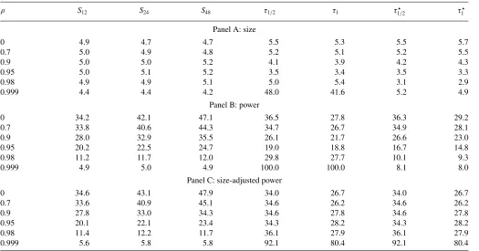
Table 1presents the simulation results for the strictly station-ary AR(1) model and set of alternatives given in M¨uller (2014). As in M¨uller (2014), we set σ2
η =1. The first three columns present the size, power, and adjusted power (we show size-adjusted power so the results for theSqtest are comparable to the tables in M¨uller (2014). Size-adjusted power for theτbstatistic is (nearly) the same as inference when the value ofcis known and so should be interpreted with this in mind) for theSq test withq =12,q =24, andq =48. The next two columns pro-vide the results for the Bonferroni-based procedure with critical values formed under the assumption that the initial condition is negligible (written asτb). As an additional point of comparison, the final two columns report results for the Bonferroni-based procedure with the limiting distributions constructed under a stationary initial condition (sincec >0 in this case, we imple-mented the testing procedure by setting the lower and upper critical values forμequal to−∞and∞, respectively, when-ever the confidence interval formed forcincluded the smallest value in our grid. This approach thus requires a user-defined minimum value ofc. In our simulations, we chosecmin=0.01)
(written asτ⋆
b). The “S-Bonf-Adj” critical values are formed withβ =0.15 (i.e., nominal coverage of the parametercequal to 1−β). To form confidence intervals forc, we invert an
ordi-nary least square (OLS)-based augmented Dickey–Fuller (ADF) test with lag length chosen by the modified Akaike information criterion (MAIC) of Perron and Qu (2007). Refinements of our procedure could include shifting to the “S-Bonf-Min” critical values of McCloskey (2012), a different choice of confidence interval for the local-to-unity parameter or an alternative test statistic toτ. However, we prefer this formulation for simplicity of interpretation. All results are based on 20,000 simulations.
The results of Table 1 are instructive on how to interpret properties of theSq test. First, theτbtest statistic controls size away from values ofρclose to one, but is severely size distorted whenρ=0.999. This reflects the fact that the critical values for τbare constructed under the assumption that the initial condition is negligible. Meanwhile, theτ⋆
b test statistic controls size well across this grid of values of ρ. The power of the τ⋆
1/2 test is
comparable to that of theS12test. However, theS24andS48tests
have higher power whenρ moves away from one. InTable 2, we again consider the AR(1) specification but use the fixed initial condition ε0=0. The pattern of the results is similar
to that of Table 1except that theτb test statistic controls size even in cases where the error terms are highly persistent. We can also contrast the results from Tables1and2to those using the least-favorable critical value. In this setting, because critical values forτbgrow asc↓0, choosing to use the least-favorable critical value produces severely undersized tests for all areas of the parameter space except whenρis very close to one.
InTable 3, we present results for the “AR(1) + noise” spec-ification and set of alternatives given in M¨uller (2014). As in M¨uller (2014), we set the variance of the additive noise term to 4. Similar toTable 1, theτbtest is oversized whenρis near one with excessive size distortion whenρ =0.999. In contrast, the τb⋆test controls size well across the grid ofρvalues and theτ1⋆/2
Table 2. AR(1),ε0=0
ρ S12 S24 S48 τ1/2 τ1 τ1⋆/2 τ
⋆
1
Panel A: size
0 4.8 4.8 4.8 5.6 5.4 5.5 5.7
0.7 5.0 4.9 4.8 5.3 5.1 5.3 5.5
0.9 5.3 5.1 5.5 4.2 4.0 4.4 4.5
0.95 5.4 5.4 5.6 3.6 3.5 3.5 3.4
0.98 5.0 4.8 5.0 4.1 4.7 3.3 3.0
0.999 2.5 2.4 2.3 6.0 5.3 3.0 2.5
Panel B: power
0 34.5 42.5 47.3 36.7 28.0 36.4 29.3
0.7 34.3 41.3 44.9 35.2 27.2 35.4 28.5
0.9 29.7 35.1 37.7 27.1 22.4 27.6 23.9
0.95 22.9 25.7 28.1 20.1 20.1 17.6 15.9
0.98 13.8 14.9 15.6 34.0 32.5 11.0 10.4
0.999 5.2 5.3 5.1 100.0 100.0 8.3 8.2
Panel C: size-adjusted power
0 35.0 43.1 48.1 34.3 27.5 34.3 27.5
0.7 34.4 41.6 45.8 34.9 27.4 34.9 27.4
0.9 28.9 34.5 35.5 35.7 28.7 35.7 28.7
0.95 21.6 23.9 25.4 37.7 29.9 37.7 29.9
0.98 13.8 15.9 15.4 48.7 38.1 48.7 38.1
0.999 10.2 12.6 11.1 100.0 100.0 100.0 100.0
statistic has comparable power properties to that of theS12test.
TheS24andS48tests suffer from size distortion for larger values
ofρas discussed in M¨uller (2014).Table 4reports the compan-ion results under a zero initial conditcompan-ion. As inTable 3, theS12
test and theτb⋆ control size well across these values ofρ. The S24 andS48 tests show some size distortion asρmoves above
0.90 whereas theτbtest controls size except whenρ=0.999.
There are three main observations from the limited sim-ulation evidence we present. First, it is instructive to see where power is directed by the Sq test. In particular, the
Sq test has little power when ρ is near 1 but much higher power elsewhere. From a practitioner’s perspective, this is a very appealing property (see next section) as the test controls size well in exactly the region of the parameter space where
Table 3. AR(1) + Noise,ε0∼N 0, ση2/(1−ρ2)
ρ S12 S24 S48 τ1/2 τ1 τ1⋆/2 τ1⋆
Panel A: size
0 4.9 5.0 5.0 5.5 5.3 5.4 5.5
0.7 4.9 4.9 5.6 5.2 4.9 5.2 5.1
0.9 5.1 5.9 9.2 4.9 4.2 5.0 4.3
0.95 5.2 6.7 12.4 4.7 4.3 4.7 4.0
0.98 5.3 7.0 15.0 5.9 6.0 4.0 3.2
0.999 4.9 7.4 17.0 48.1 41.9 4.8 4.5
Panel B: power
0 34.4 42.7 47.2 35.5 27.1 35.1 27.9
0.7 34.1 42.5 49.1 33.9 26.3 33.7 26.8
0.9 28.7 37.9 53.7 27.1 22.8 26.7 21.6
0.95 22.0 29.8 50.0 21.2 20.7 17.6 14.7
0.98 12.4 17.8 37.3 30.9 28.7 9.6 8.6
0.999 5.5 8.4 19.4 100.0 100.0 6.8 6.7
Panel C: size-adjusted power
0 34.8 42.7 47.3 34.4 26.2 34.4 26.2
0.7 34.6 42.9 47.0 36.2 26.9 36.2 26.9
0.9 28.3 34.1 38.0 35.7 29.1 35.7 29.1
0.95 21.2 23.0 25.4 35.0 28.2 35.0 28.2
0.98 11.5 11.9 12.0 36.6 28.4 36.6 28.4
0.999 5.7 5.7 5.6 92.4 80.6 92.4 80.6
Table 4. AR(1) + Noise,ε0=0
ρ S12 S24 S48 τ1/2 τ1 τ1⋆/2 τ
⋆
1
Panel A: size
0 4.9 4.9 5.0 5.5 5.3 5.4 5.6
0.7 4.9 4.9 5.5 5.2 4.9 5.1 5.1
0.9 5.3 6.0 9.6 4.9 4.5 5.0 4.6
0.95 5.6 7.1 12.6 4.7 4.4 4.6 4.1
0.98 5.4 6.9 14.7 5.4 5.5 4.5 3.6
0.999 2.9 4.0 9.8 7.1 6.3 3.7 2.8
Panel B: power
0 34.5 42.8 47.3 35.5 27.2 35.2 27.9
0.7 34.5 43.0 49.5 34.2 26.6 34.0 27.1
0.9 30.5 40.1 55.4 28.2 24.0 27.6 22.6
0.95 24.7 33.6 54.4 22.5 22.3 18.5 15.8
0.98 15.4 22.4 44.5 35.0 33.6 10.2 9.6
0.999 5.9 8.7 20.3 100.0 100.0 6.9 6.8
Panel C: size-adjusted power
0 34.8 43.1 47.2 34.4 26.1 34.4 26.1
0.7 34.9 43.2 47.0 36.7 27.4 36.7 27.4
0.9 29.3 35.9 39.6 36.4 28.4 36.4 28.4
0.95 22.8 25.3 27.4 37.9 30.2 37.9 30.2
0.98 14.1 14.6 15.5 47.7 38.3 47.7 38.3
0.999 10.1 11.6 10.7 100.0 100.0 100.0 100.0
inference is most difficult. Second, the results show clearly that the underlying assumption of how the initial condition is gener-ated plays a key role in the performance of testing procedures for large values of ρ. In particular, procedures that may per-form well in terms of size control when the initial condition is negligible can have severe size distortion when the initial con-dition is drawn from its unconcon-ditional distribution. This is not a surprising result, but one that may not be fully appreciated outside of the unit root testing literature. Third, the simulations show that the choice ofqcan matter and so further guidance for applied practitioners would be an important contribution for future work.
3. APPLICATION: LONG-HORIZON RETURN PREDICTABILITY
Conventional wisdom in applied time series would suggest the presence of model misspecification when products of esti-mated error terms are highly persistent. The consummate exam-ple would be the omission of the lagged left-hand side variable in the canonical spurious regression case. However, an impor-tant situation where the prescription to add lags of the dependent variable is unavailable is in long-horizon predictability regres-sions, such as predictingh-period ahead stock and bond returns. We revisit the question of longer-horizon return predictability for equities and bonds using theSq test. These two simple em-pirical exercises demonstrate clearly the applicability of the new testing procedure.
Long-horizon stock return predictability has been studied by a number of authors (see, e.g., Koijen and Nieuwerburgh2011or Rapach and Zhou2013for general discussions.) Here, we follow
the standard approach in the literature and form continuously compounded, cumulative stock returns as
rxt+h= h
j=1
rxt+j, (3.1)
where rxt is the 1 month compounded excess return formed as the Center for Research in Security Prices (CRSP) value-weighted return less the 1 month interest rate (here mea-sured as the Fama–Bliss risk-free rate). We consider two regressors: (1) the log dividend yield formed as the nat-ural logarithm of the sum of monthly dividends over the last 12 months relative to the current price and (2) the Fama–Bliss risk-free rate. We include the latter regressor as Ang and Bekaert (2007) argued that the predictive ability of the div-idend yield is enhanced by including this variable. We consider two sample periods: monthly data over the period 1952–2012 and over the period 1952–1990. We include the latter, shorter sample, as it is perceived that the dividend yield was a more reliable predictor of stock returns up to 1990. Finally, we report results for values of h∈ {6,12,24,36} months. Because the returns in Equation (3.1) are calculated with overlapping peri-ods, they have a considerable degree of persistence, comparable to that of the right-hand side variables. Thus, concerns have arisen about conducting inference in such a setting.
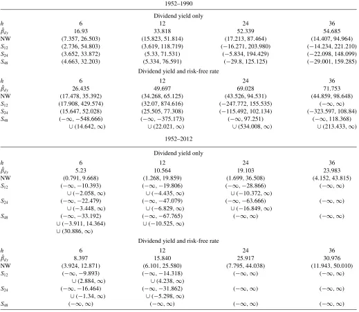
Confidence intervals formed using Newey–West (NW) stan-dard errors with lag truncation parameter h and those using M¨uller (2014) are reported inTable 5. When the sample is re-stricted to 1952–1990,theSq test provides evidence of return predictability at shorter horizons, although the confidence inter-vals vary considerably depending on the specification and the choice of q. However, there is little evidence of predictability
Table 5. Long-horizon regressions: Equity returns
1952–1990
Dividend yield only
h 6 12 24 36
ˆ
βdy 16.93 33.818 52.339 54.685
NW (7.357,26.503) (15.823,51.814) (17.213,87.464) (14.407,94.964) S12 (2.736,54.803) (3.619,118.719) (−16.271,203.980) (−14.234,221.210)
S24 (3.652,33.872) (5.33,71.531) (−5.834,194.429) (−22.098,148.099)
S48 (4.663,32.203) (5.334,76.591) (−29.8,125.125) (−29.001,159.285)
Dividend yield and risk-free rate
h 6 12 24 36
ˆ
βdy 26.435 49.697 69.028 71.753
NW (17.478,35.392) (34.268,65.125) (43.526,94.531) (44.859,98.648) S12 (17.908,429.574) (32.07,874.616) (−247.772,155.535) (−∞,∞)
S24 (15.647,52.028) (25.505,77.308) (−115.492,102.134) (−323.597,108.84)
S48 (−∞,−548.666) (−∞,−375.173) (−∞,97.251) (−∞,118.368)
∪(14.642,∞) ∪(22.021,∞) ∪(534.008,∞) ∪(213.433,∞) 1952–2012
Dividend yield only
h 6 12 24 36
ˆ
βdy 5.23 10.564 19.103 23.983
NW (0.791,9.668) (1.268,19.859) (1.699,36.508) (4.152,43.815)
S12 (−∞,−10.393) (−∞,−19.806) (−∞,−28.866) (−∞,∞)
∪(−2.058,∞) ∪(−4.435,∞) ∪(−10.372,∞)
S24 (−∞,−22.479) (−∞,−47.079) (−∞,−63.666) (−∞,∞)
∪(−3.448,∞) ∪(−6.829,∞) ∪(−16.849,∞)
S48 (−∞,−33.192) (−∞,−67.765) (−∞,∞) (−∞,∞)
∪(−3.911,14.364) ∪(−10.525,∞)
∪(30.886,∞)
Dividend yield and risk-free rate
h 6 12 24 36
ˆ
βdy 8.397 15.840 25.917 30.976
NW (3.924,12.871) (6.101,25.580) (7.795,44.038) (11.943,50.010)
S12 (−∞,−9.893) (−∞,−14.318) (−∞,∞) (−∞,∞)
∪(2.884,∞) ∪(4.238,∞)
S24 (−∞,−16.464) (−∞,−31.862) (−∞,∞) (−∞,∞)
∪(−1.34,∞) ∪(−5.298,∞)
S48 (−∞,∞) (−∞,∞) (−∞,∞) (−∞,∞)
NOTE: This table shows the results for long-horizon predictability regressions of equity market returns on the log dividend yield and the risk-free rate. ˆβdyis the OLS coefficient
corresponding to the log dividend yield. Newey–West (NW) standard errors are constructed withhlags. All confidence intervals have nominal coverage of 95%.
at shorter horizons for the full sample. At longer horizons there is no evidence of predictability for either the restricted or full sample based on theSqtest.
Next, we consider a similar exercise for excess bond returns. Specifically, we revisit the influential work of Cochrane and Piazzesi (2005,2008), where the authors form a bond-return forecasting factor using linear combinations of forward rates. To proceed, we first must form this return-forecasting factor (hereafter, CP factor). We use excess returns and log forward rates, defined by
rxt(+n)1 ≡pt(+n−11)−pt(n)−yt(1), f
(n)
t ≡p
(n−1)
t −p
(n)
t ,
wherept(n)is the log price of annyear discount bond at timet andyt(1)is the 1-month GSW rate (GSW refers to zero-coupon bond yields from Gurkaynak, Sack, and Wright (2007), which
are available at a daily frequency on the Board of Governors of the Federal Reserve’s research data page). We use GSW yields to construct excess returns and Fama–Bliss forward rates as re-gressors. We follow Cochrane and Piazzesi (2008) and regress 14 excess returnsrxt+1=[rxt(2)+1, rx
(3)
t+1, . . . , rx (15)
t+1]
′on a
con-stantzt =1 and five forward rateswt =[yt(1), f
(2)
t , . . . , f
(5)
t ]′. Cochrane and Piazzesi (2008) formed the CP factor by tak-ing the first principal component of the fitted values from this regression. It can be shown that this is equivalent to the maximum-likelihood estimator (MLE) of a reduced-rank re-gression (with coefficient matrix of rank one) under the as-sumption of iid Gaussian errors and a scalar variance ma-trix. We also consider a weighted version of the CP factor, formed as the MLE under the assumption of a diagonal vari-ance matrix (see Adrian, Crump, and Moench2014for further details).
Table 6. Long-horizon regressions: Bond returns
Identity weight matrix
In-sample Out-of-sample (5 years) Out-of-sample (10 years) Out-of-sample (15 years) ˆ
βCP 0.220 0.052 0.082 0.063
NW (0.101,0.339) (−0.001,0.105) (0.047,0.117) (−0.009,0.136)
βCP 0.231 0.053 0.086 0.066
NW (0.105,0.356) (−0.003,0.108) (0.049,0.122) (−0.012,0.144) S12 (−∞,0.355)∪(2.257,∞) (−∞,∞) (−∞,∞) (−∞,∞)
S24 (−0.116,0.342) (−0.155,0.209) (−∞,0.132)∪(0.226,∞) (−∞,−13.464)∪(−0.035,∞)
S48 (−0.107,0.376) (−0.178,0.134) (−∞,−0.205)∪(−0.045,0.13)∪(0.419,∞) (−0.078,0.843)
NOTE: This table shows the results for long-horizon predictability regressions of 1 year excess holding period returns on the CP factor. ˆβCPis the OLS coefficient corresponding to the
CP factor. The first column report results for the CP factor constructed on data for 1971–2012. The next three columns report results for the CP factor constructed in real time with a 5, 10, and 15 year burn-in period, respectively. Newey–West (NW) standard errors are constructed with 12 lags. All confidence intervals have nominal coverage of 95%.
We then regress average excess returns on the CP factor,
rxt+1=α+βxt+ǫt,
We use theSq test statistic to construct confidence intervals (results reported in Table 6). We then repeat the exercise but now we construct the CP factor without using future information after a certain burn-in period. (We also considered specifications that added the term spread as an additional predictor. The results in this case were qualitatively similar to those presented here.) We find that the conclusions drawn from the confidence intervals formed from theSq test are sensitive to different values of q and different burn-in periods. As in the equity application, we find that confidence intervals can be asymmetric, sometimes disjoint but nonempty (as discussed in M¨uller2014). Despite this, we find no evidence that a predictive relationship can be uncovered with these data.
ACKNOWLEDGMENTS
The authors thank Lutz Kilian, Adam McCloskey, Emanuel Moench, and Ulrich M¨uller for helpful comments and discus-sions and the editors, Keisuke Hirano and Jonathan Wright, for inviting us to participate in this intellectual exchange. Benjamin Mills provided excellent research assistance. The first author gratefully acknowledges financial support from the National Science Foundation (SES 1122994). The views expressed in this article are those of the authors and do not necessarily rep-resent those of the Federal Reserve Bank of New York or the Federal Reserve System.
REFERENCES
Adrian, T., Crump, R. K., and Moench, E. (2014), “Regression-based Estimation of Dynamic Asset Pricing Models,” Staff Report 493, Federal Reserve Bank of New York. [328]
——— (2009), “Hybrid and Size-corrected Subsampling Methods,” Economet-rica, 77, 721–762. [325]
Andrews, D. W. K., and Guggenberger, P. (2010), “Asymptotic Size and a Problem with Subsampling and with themOut ofnBootstrap,”Econometric Theory, 26, 426–468. [325]
Ang, A., and Bekaert, G. (2007), “Stock Return Predictability: Is it There?,” Review of Financial Studies, 20, 651–707. [327]
Atchad´e, Y. F., and Cattaneo, M. D. (2014), “A Martingale Decomposition for Quadratic Forms of Markov Chains (with Applications),”Stochastic Processes and Their Applications, 124, 646–677. [324]
Cochrane, J., and Piazzesi, M. (2005), “Bond Risk Premia,”American Economic Review, 95, 138–160. [328]
——— (2008), “Decomposing the Yield Curve,” Working Paper, University of Chicago. [328]
Elliott, G., M¨uller, U. K., and Watson, M. W. (2013), “Nearly Optimal Tests When a Nuisance Parameter is Present Under the Null Hypothesis,” Working Paper, Princeton University. [324]
Gurkaynak, R. S., Sack, B., and Wright, J. H. (2007), “The U.S. Treasury Yield Curve: 1961 to the Present,”Journal of Monetary Economics, 54, 2291–2304. [328]
Kiefer, N. M., and Vogelsang, T. J. (2005), “A New Asymptotic Theory for Heteroskedasticity-autocorrelation Robust Tests,”Econometric Theory, 21, 1130–1164. [324]
Koijen, R. S., and Nieuwerburgh, S. V. (2011), “Predictability of Returns and Cash Flows,”Annual Review of Financial Economics, 3, 467–491. [327] McCloskey, A. (2012), “Bonferroni-Based Size-Correction for Nonstandard
Testing Problems,” Working Paper, Brown University. [325]
M¨uller, U. K. (2014), “HAC Corrections for Strongly Autocorrelated Time Series,” Journal of Business and Economic Statistics, 32, 311–322. [324,325,327,329]
Perron, P., and Qu, Z. (2007), “A Simple Modification to Improve the Finite Sample Properties of Ng and Perron’s Unit Root Tests,”Economics Letters, 94, 12–19. [325]
Rapach, D. E., and Zhou, G. (2013), “Forecasting Stock Returns,” inHandbook of Economic Forecasting (Vol. II), eds. G. Elliott and A. Timmermann, Amsterdam: North-Holland, pp. 329–383. [327]
Tanaka, K. (1996),Time Series Analysis: Nonstationary and Noninvertible Dis-tribution Theory, New York: Wiley. [324]