Calculation of 20 kV Distribution Network Energy Losses and
Minimizing Effort Using Network Reconfiguration in Region of
PT PLN (Persero) UPJ Bantul
Slamet Suripto
*11Department of Electrical Engineering, Universitas Muhammadiyah Yogyakarta
Jl Lingkar Selatan Tamantirto Kasihan Bantul, (0274)387656 *Corresponding author, e-mail: [email protected]
Abstract – Power distribution system is a component of electric power system to deliver electricity energy from substation to customer location. In power distribution system, there are some power loss was changed as heat. Power distribution losses is a natural occurrence, so one gets to be done only minimize to support global energy efficiency. The way to reduce power loss in the power distribution system is by reconfiguration the existing line. Reconfiguration means a process of operating the switch (NO and NC) and change the topology line. Then, power loss in the power distribution system is computed
with “ETAP” simulation software. From computing result of distribution network losses on existing line at PT. PLN UPJ. Bantul BNL 6, BNL 7 and BNL 11 feeders are gotten energy losses as 2,669,328 kWh per year or 1.72 %. Network reconfiguration that involves BNL 6, BNL 7 and BNL 11 feeder gets energy losses decrease as 1.00 % per year. Copyright © 2017 Universitas Muhammadiyah Yogyakarta- All rights reserved.
Keywords: Distribution system, energy losses, reconfiguration, efficiency
I.
Introduction
Distribution of electricity through the distribution network from substations to loads give results in energy lost on the channel since turned into heat. This energy lost is called losses or network energy losses. Losses are naturals, and then cannot be avoided. Losses are energy lost experienced by providers that eventually to be borne by consumers in form of energy price which is increasing. Therefore efforts are needed to minimize energy lost to support global energy efficiency and cheap electricity price for consumers.
As an illustration, energy lost that occurs in region PT. PLN APJ Yogyakarta or Yogyakarta Province in 2005 until 2009 recorded an average of 9 %. For 2009, energy lost in APJ Yogyakarta was 160,825,155 kWh. Energy lost in Bantul Regency was an average of 9.65 % that is 15,519,316 kWh.
II.
Literature Review
Distribution network that connects distribution transformer with low-voltage consumers called Low-voltage Distribution Networks (JTR) or Secondary Distribution Networks. LDN/JTR that serves huge loads usually use 3-phase 4-wire network with voltage of 380 volt between phases. As for small load services, includes households, using single-phase 2-wire network with voltage of 220 volt phase to neutral.
Weakness on radial system could be overcome using ring or loop system, which is aligned to be connected between adjacent feeders. If there is disturbance on one of the feeders, loads could be diverted to other adjacent feeders by opening/closing the separator switch (ABSW). Management certainly more complicated and also more expensive construction costs, but result in better services.
2.1 Distribution Network Performance
Distribution network performance is related in the quality of electric power that can be served by the distribution network. The quality includes voltage fluctuations up to consumers and the continuity of service. Another thing that should be considered was power loss on network. The power loss will determine efficiency of the distribution network.
2.2 Calculation of Network Energy Losses
Distribution Network energy losses is differences between energy that sent from substation to distribution network with the amount of energy sold to consumers. For feeders, energy losses are differences between energy measured at the substation by the number of kWh sold to consumers connected to the feeders. Energy losses usually expressed as percentage of energy losses of incoming energy to the grid.
(1)
(2)
Energy losses is certain on management of electrical energy, so the effort is reduce the amount of energy losses becomes more efficient. Network energy losses divided into two:
a. Technical energy losses
Technical energy losses are power loss that occurs naturally because of the current flows in network and equipments. This power loss is defined as square of the current flows on network and its equipments multiplied by its resistance. This includes loss of power in Medium-voltage Distribution Network (MDN/JTM), transformers,
JTR/LDN, and other equipment used on the network.
b. Non-technical energy losses
Non-technical energy losses are caused by errors of measurements and recording, and not good in monitoring of energy usage. Efforts that can be done are improving the accuracy of measurement system, records administrative, and supervision of illegal electrical energy consumption.
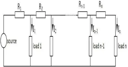
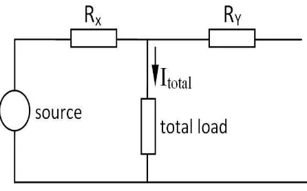
2.3 Equivalent Circuit
Equivalent circuit need to be made to simplify the circuit analysis when calculating technical energy losses of MDN/JTM which generally have a load attached to transformers. It also required when drawing and simulating circuit diagram in application program. The equivalent circuit is created by collecting all the existing loads then put it at a certain distance from the sources. Distance of load from this source should be selected so that analytical results obtained through equivalent circuit approach the results obtained from the source. This resistance value (RX) is resistance that passed by total load currents, which would affect value of power losses in circuit resistance. The value RX should be selected in order to value of power losses in circuit resistance approach the value of power losses from the original circuit.
Fig. 2. Equivalent circuit
From calculation it was found that the percentage of the exact RX for equivalent circuit is not equal to the number of loads of different circuit, as shown on Table 1. Percentage of RX in the table below is comparison between RX resistance against total circuit resistance (RX + RY).
Table 1. R
Xpercentage in equivalent circuit
No. Number of loads RX percentage
From the calculation above obtained that if the circuit consists of 3 loads, then the value of RX is done to achieve the desired end result according to the procedure below.
1. Collection of physical network data, loads for each feeders, and current curve of daily load of feeders.
2. Loads grouping for each sections of the feeders and data collection of transformers capacity on installed loads.
3. Simulations of network for several load conditions and network configurations. 4. Simulations of power flow and calculate
network energy losses of every condition. 5. Forecasting of load growth and evaluate the
network capacity of each feeders.
IV.
Results and Discussion
Reconfiguring of distribution network is a change of network compositions in order to raise the network performance. This reconfiguration can be done within several ways, namely:
a. Moving loads from certain feeders to
From the results by regrouping of feeder’s loads
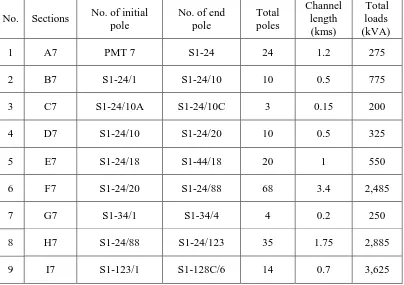
data BNL-6, BNL-7, and BNL-11 could be drawn the channel length and total loads (kVA installed) in each sections that shown in Table 2, Table 3, and Table 4.
Table 2. Length and amount of installed loads for each section in BNL 6 feeder
5 E6 S6-38 S6 -94 56 2.8 1,520
6 F6 S6-94A S6-94K 15 0.75 365
7 G6 S6 -94 S6 -113 17 0.85 550
8 H6 S6 -113 S6 -144 31 1.55 425
9 I6 S6 -143A S6 -143/26 26 1.3 250
10 J6 S3-27/59 S3-125Z/45 18 0.9 475
11 K6 S3-125Z/45 S3-125Z/75 30 1.5 650
12 L6 S3-125Z/75 S3-125Z/90 15 0.75 725
13 M6 S3-125Z/38 S3-125Z/90 42 2.1 1,250
14 N6 S3-125Z/90
S3-125Z/141 51 2.55 635
15 O6
S3-125Z/141
S3-125Z/151 10 0.5 -
16 P6
S3-125Z/151
S3-125Z/199 48 2.4 1,925
17 Q6
S3-125Z/75A S3-75X 25 1.25 550
18 R6 S3-125Z S3-157 27 1.35 500
19 S6 S3-75X/1 S3-75X/11 10 0.5 1,125
20 T6 S3-75X/11 S3-75X/89 78 3.9 1,175
Total 13,530
Table 3. Length and amount of installed loads for each section in BNL 7 feeder
No. Sections No. of initial pole
No. of end pole
Total poles
Channel length
(kms)
Total loads (kVA)
1 A7 PMT 7 S1-24 24 1.2 275
2 B7 S1-24/1 S1-24/10 10 0.5 775
3 C7 S1-24/10A S1-24/10C 3 0.15 200
4 D7 S1-24/10 S1-24/20 10 0.5 325
5 E7 S1-24/18 S1-44/18 20 1 550
6 F7 S1-24/20 S1-24/88 68 3.4 2,485
7 G7 S1-34/1 S1-34/4 4 0.2 250
8 H7 S1-24/88 S1-24/123 35 1.75 2,885
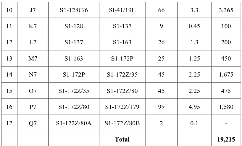
10 J7 S1-128C/6 SI-41/19L 66 3.3 3,365
11 K7 S1-128 S1-137 9 0.45 100
12 L7 S1-137 S1-163 26 1.3 200
13 M7 S1-163 S1-172P 25 1.25 450
14 N7 S1-172P S1-172Z/35 45 2.25 1,675
15 O7 S1-172Z/35 S1-172Z/80 45 2.25 475
16 P7 S1-172Z/80 S1-172Z/179 99 4.95 1,580
17 Q7 S1-172Z/80A S1-172Z/80B 2 0.1 -
Total 19,215
Table 4. Length and amount of installed loads for each section in BNL 11 feeder
No Sections No. of initial pole
No. of end pole
Total poles
Channel length (kms)
Total loads (kVA)
1 A11 PMT 11 S3-2/88 88 4.4 3,495
2 B11 S3-2/88 S3-2/122 34 1.7 1,560
3 C11 S3-2/122 S3-2/149 27 1.35 700
4 D11 S3-2/149 S3-2/248 99 4.95 1,350
5 E11 S3-2/248 S3-2/255 7 0.35 -
6 F11 S3-2/255 S3-2/299 44 2.2 500
7 G11 S3-2/299A S3-2/299R 18 0.9 375
8 H11 S3-2/353 S3-2/364 11 0.55 75
9 I11 S3-2/364 S3-2/462 98 4.9 950
10 J11 S3-2/122 S1-5C/13 16 0.8 160
11 K11 S3-149/1 S3-149/3 3 0.15 -
12 L11 S3-255/1 S3-255/3 3 0.15 1,250
13 M11 S3-299/1 S3-299/47 47 2.35 610
14 N11 S3-299N/1 S3-299N/24 24 1.2 875
15 O11 S3-364 S3-364/54 54 2.7 350
17 Q11 S3-248 S3-248/34H 42 2.1 1,540
18 R11 S6-193 S6-218 25 1.25 175
19 S11 S6-193/1 S6-193/57 57 2.85 875
20 T11 S6-193 S6-177 16 0.8 150
21 U11 S6-144 S6-177 33 1.65 290
22 V11 S6-177/1 S6-177/83 83 4.15 1,435
23 W11 S6-83/1 S6-83/32 32 1.6 1,605
TOTAL 19,470
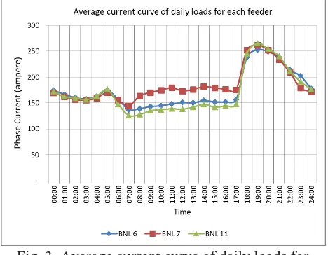
To determine the level of feeder loads, it needed the average curve of current of daily loads for each feeder. Daily loads curve for BNL-6, BNL-7, and BNL-11 feeders at November 17th 2011 shown at Figure 3.
Fig. 3. Average current curve of daily loads for each feeder
From load curve in the picture above, calculation of percentage of loading at Peak Load Time (WBP) and Normal Load Time (LWBP), as shown in Table 5.
Table 5. Percentage of loading in feeders at WBP and LWBP
Loading Time Feeders
6 7 11
WBP 69 % 50 % 50 %
LWBP 40 % 34 % 26 %
Next step is simulation in “ETAP” software
with drawing the network and installed loads in existing condition. Program runs with WBP and LWBP loading scenario. From network power flow simulation, results load current, load power, and losses for each network at WBP and LWBP scenario in existing condition as shown in Table 6 and Table 7.
Table 6. Load current, Load power, and network losses at WBP
Feeders BNL 6 BNL 7 BNL 11 Total % of
Loading 69 % 50% 50 %
Power
(kW) 8,643 9,023 8,881 26,547 Current
(A) 264.7 275.2 277.4
Losses
(kW) 219.4 190.4 246.4 656.2 End-point
Voltage (kV)
20,212 20,197 19,855
Table 7. Load current, Load power, and Network losses at LWBP
Feeders BNL 6 BNL 7 BNL 11 Total
% of
Loading 40 % 34 % 26 % Power
(kW) 5,197 6,274 4,818 16,289 Current
(A) 157.4 189.9 148.3 Losses
(kW) 77.8 90.8 70.9 239.5 End-point
Voltage (kV)
Several chances of reconfiguring the distribution network with moving loads from feeders that includes BNL 6, BNL 7, and BNL 11 feeders are shown in Table 8.
To identify total network losses for each configuration, it did a power flow simulation. From the simulation can be drawn as shown on table 9.
Calculation of network energy losses done for several configuration conditions, and then the results are compared with existing condition. For complete calculation are shown on table 10.
Table 8. Chances of reconfiguring the distribution network at BNL 6, BNL 7, and BNL 11 feeders
No. Condition Feeders Section
Existing Position
New Position
ABSW Condition Changes
1 Configuration 1 O7 and P7 BNL 7 BNL 11 S1-172Z/35 OFF S3-255/3 ON
2 Configuration 2 M6 and N6
Connected with I6
Connected with L6
S3-125Z/90 ON S3-125Z/141 OFF
3 Configuration 3 H6 and I6 Connected with G6
Connected with L6
S6-142 OFF S3-125Z/90 ON
Table 9. Power and network losses at several configuration conditions of network
No. Condition
Network Power (kW)
Input Losses
WBP LWBP WBP LWBP
1 Existing 26,547 16,289 656.2 239.5 2 Configuration 1 26,495 16,277 672.8 243 3 Configuration 2 26,566 16,295 649.8 237.1
4 Configuration 3 26,515 16,278 667.7 243.7
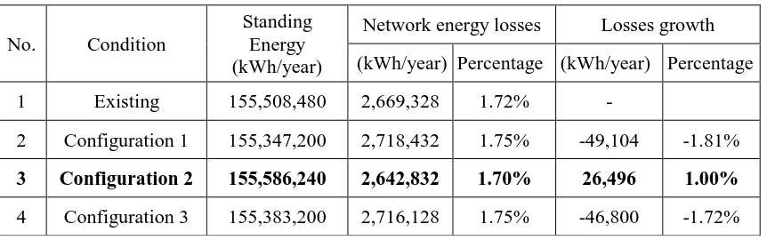
Table 10. Energy losses in several configuration conditions of network
No. Condition
Standing Energy (kWh/year)
Network energy losses Losses growth
(kWh/year) Percentage (kWh/year) Percentage
1 Existing 155,508,480 2,669,328 1.72% -
2 Configuration 1 155,347,200 2,718,432 1.75% -49,104 -1.81%
3 Configuration 2 155,586,240 2,642,832 1.70% 26,496 1.00%
4 Configuration 3 155,383,200 2,716,128 1.75% -46,800 -1.72%
It can be drawn from calculation that at existing condition, energy that come to BNL 6, BNL 7, and BNL 11 feeders are 155,508,480 kWh per year. Energy losses that exist in this condition are 2,669,328 kWh or 1.72 % per year. Chance of reconfiguration that have smallest energy losses is
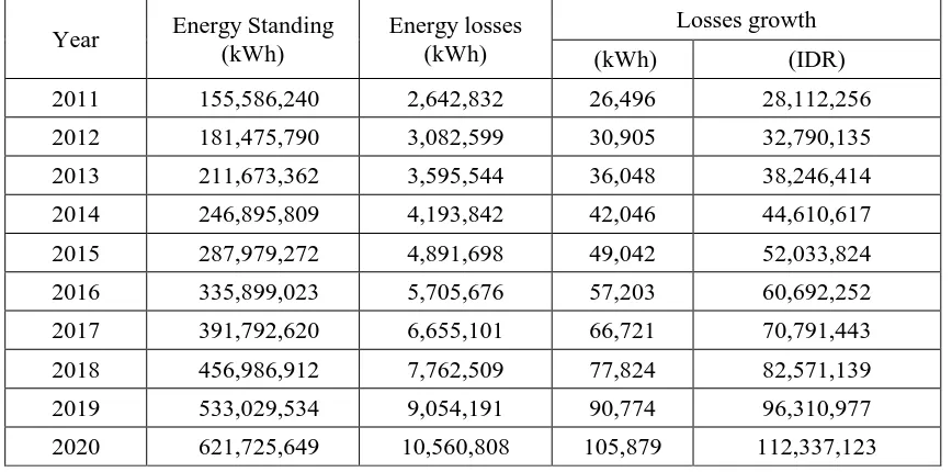
that basic recommendation price (HPP) in 2012 are IDR 1,061 per kWh (RUPTL 2011-2020), then from the configuration we have savings IDR 28,112,256 per year.
Prediction of loads growth in Bantul Regency is adjusted with projection of national electricity and DI Yogyakarta Province. Growth rate of installed kVA for DI Yogyakarta in 1999 to 2009 are 6.47 % per year. Growth rate of installed kVA in Bantul
From the data above are predicted that average
growth loads in UPJ Bantul, includes feeder’s loads
that been observed are equal with average growth loads in DI Yogyakarta province which is 8 %.
Growth rate of 8 % is a number of peak loads growth denominated in megawatt (MW). With this growth number, then current that flow in network approximately also raise 8 % per year. The value of network power losses equal with squared value of current flowing, so that network power losses
growth are become 16.64 % per year. With value of power losses of 16.64 %, estimation of energy savings at configuration 2 condition until 2020 are shown in table 12.
Table 11. Peak Loads Growth Projections
Year National Peak
Table 12. Projection of energy savings per year in configuration 2
Year Energy Standing
Distribution Network energy losses in UPJ Bantul BNL 6, BNL 7, and BNL 11 feeders in existing condition are 2,669,328 kWh per year or 1.72 %. Network reconfiguring for BNL 6, BNL 7, and BNL 11 feeders can reduce network energy losses for 26,496 kWh or 1.00 % that means there is
changing the one-phase network becoming three-phase networks.
References
[1] Abdul Kadir, 1996, Pembangkit Tenaga Listrik, UI-Press, Jakarta.
[2] Anonim, 2003, Laporan Pembuatan Master Plan Sistem Distribusi 20 kV untuk APJ Yogyakarta dan APJ Surakarta, PT. PLN (Persero) Distribusi Jateng - DIY dan Jurusan Teknik Elektro Fakultas Teknik UGM
[3] Anonim, 2000, Persyaratan Umum Instalasi Listrik 2000, Badan Standar Nasional, Jakarta
[4] Anonim, 2011, Rencana Usaha Penyediaan Tenaga Listrik 2011- 2020, PT. PLN (Persero), Jakarta [5] Billinton, Roy, & Allan, Ronald N, 1996, Reliability
Evaluation of Power System, Plenum Press, New York.
[6] Citarsa, Ida Bagus Feri, 2007, Perencaan Rekonfigurasi Jaringan Distribusi untuk Reduksi Rugi Daya, Tesis Teknik Elektro UGM
[7] Ginting, Tenang Ebenezer, 2007, Perhitungan Susut Distribusi Berdasar Profil Beban, Tesis Teknik Elektro UGM
[8] Haryadi, Rekonfigurasi Jaringan Tegangan Menengah 20 kV PT. PLN (Persero) UPJ. Wates untuk Memperkecil Susut Teknik, Tesis Teknik Elektro UGM
[9] Munthe, Barayan, 2005, Studi Kinerja Jaringan Distribusi Dan Perkiraan Pertumbuhan Beban, Tesis Teknik Elektro UGM
[10] Rahmanto, Danang, 2008, Susut Energi Listrik pada Sistem Distribusi Berdasar Perhitungan dan Pengukuran, Teknik Elektro UI
[11] Willis, H. Lee, 2004, Power Distribution Panning Reference Book, Marcel Dekker, Inc, New York. [12] Yaman, 2007, Perhitungan Susut Energi Teknik pada
Jaringan Distribusi Primer, Tesis Teknik Elektro UGM
Author information
Slamet Suripto received B.Sc. degree
from Universitas Gadjah Mada in 1987, M.Eng. degree from Department of Electrical Engineering, Universitas Gadjah Mada, Yogyakarta, Indonesia in 2012,