*Corresponding author.
CHARACTERIZATION OF RESERVOIR SANDSTONES USING
LOG ANALYSIS TECHNIQUE EXTENDED ELASTIC
IMPEDANCE IN FIELD X
Dhony Widyasandy1*, Adi Susilo2, Fatkhul Mu’in3
1Magister Program of Physics, Faculty of Mathematics and Natural Sciences, Brawijaya University
2Department of Physics, Faculty of Mathematics and Natural Science, Brawijaya University 3Department of Geophysics PT. Pertamina UTC (Upstream Technology Center), Jakarta Pusat
Recieved: 28th May 2017; Revised: 27th September 2017; Accepted: 30th October 2017
ABSTRACT
Extended Elastic Impedance (EEI) Analysis first introduced by Whitcombe (2002) was used for the predicting lithology review and fluid in a hydrocarbon reservoir. EEI is an application of an angle that is applied in a certain range until the zone of interest (ZoI) clarified. EEI is an interesting subject to observe and very useful to be applied on seismic attributes with its ability to predict lithology and fluid where acoustic impedance of sands and shale looks almost in the same pattern. Applying this method allows the result of the sand and shale anomalies to be seen in a different way. EEI has the ability to review the estimation of elastic parameters. In this research, It used multiple parameters which analyzed directly by using an original log from well that are a 𝑣𝑝/𝑣𝑠 ratio, pseudo gamma ray, pseudo NPHI, pseudo resistivity.
The results of this study indicate that the use of angle optimization on EEI can interpret the intended zone of interest.
Keywords: Pre-Stack Time Migration (PSTM); Well log analysis; AVO (Amplitude Versus Offset); EEI (Extended Elastic Impedance)
Introduction
Increasing of the human population followed with the economic growth affects an increasing need of energy. Oil and gas, usually called hydrocarbon, are still a primary energy source in the levels of industry, transport, and households which are also included as the non-renewable energy. Therefore, hydrocarbons search by studying the physical properties of rock layers using seismic methods is less effective. So, the effort to increase the production of hydrocarbons in an oil field requires a good understanding of reservoir characterization.
Extended Elastic Impedance (EEI) is an extended seismic reservoir characterization technique from Acoustic Impedance (AI) and Elastic Impedance (EI) using stack zero offset data with the principle of incident wave angle 0° or perpendicular to the reflected plane, but
in reality has limitations on estimates the presence of hydrocarbons.1 The limitation of the AI technique gives rise to a new technique of EI inversion technique which is a generalization of AI. The EI uses non-zero offset data which means that data is stacked only at a certain range of angles and refers to the principle of incident angles not equal to 0°. In EI inversion technique hydrocarbon approximation becomes more sensitive because besides influenced by density function and velocity of P wave (𝑣𝑝), also influenced by S wave velocity (𝑣𝑠).
Several studies that were conducted by Andri Fernandus3 on sandstone lithology determination using Mu-Rho EEI inversion, porosity and gamma ray; Johan Maulana Hadi4 regarding EEI inversion results and predictive analysis 𝑣𝑠 to show the strong influence of the value of the matrix elastic modulus of rock; Dyah Woelandari5 on the Lambda-Mu-Rho method has not been effective in separating fluid and lithology; Sayed Ali Gharaee Shahri6 on log data can
provide very important information in defining reservoirs with petrophysical integration and rock physics allowing to identify seismic anomalies in predicting lithology.7 Thus, with the advantages of this
EEI log analysis method it is expected to produce accurate information on a reservoir for further exploration.8
Methods
The data used in this research are seismic data of Prestack Time Migration (PSTM) XYZ Field in South Sumatra and well logs data such as gamma ray log, density log, neutron porosity log, resistivity log, P-sonic log. In addition there is data checkshot which is the result of the measurement of the travel time of seismic waves to change the time domain to domain depth in PSTM seismic data. Checkshot data consists of two variables, namely depth data and two way time data of seismic waves. For other supporting data in the form of geological data of Jambi sub basin area.
There are several stages performed for data processing. The first stage, pre-conditioning data gather PSTM includes Normal Move Out (NMO) correction, mute, bandpass filter, trim static correction and output of supergather data. The second stage, analyzed well logs data to predict 𝑣𝑠 log correction calculated from P-sonic logs with the help of Humpson-Russell software. From the supergather data the result of pre-conditioning gather output is used to create a well sensitivity analysis map which is shown through crossplot 𝑣𝑝to 𝑣𝑠. The crossplot result shows the zone of interest in this study.
The third stage, analyzes the sensitivity which is performed to find out suitable parameters in separation of lithology and fluid in reservoir. Well log analysis is adjusted to the availability of log data for each well such as 𝑣𝑝/𝑣𝑠 for depth, 𝑣𝑝/𝑣𝑠 against gamma ray,
𝑣𝑝/𝑣𝑠 against NPHI, 𝑣𝑝/𝑣𝑠 against resistivity. The crossplot result represents the zone of interest in the research area.
The fourth stage, anayze the AVO intercept and gradient (Amplitude Versus Offset) that are used to estimate the angle (𝜒 angle) of EEI. AVO is obtained from supergather data which is analyzed based on the increase of the reflected signal amplitude and increase the source wave distance to the receiver. Therefore, the supergather data of early pre-conditioning data results greatly affect the intercept and AVO gradient results.
The fifth stage, correlates the target log with the EEI derivative log after obtaining an approximate 𝜒 angle. To estimate the 𝜒 angle in the EEI process is done by selecting the target log that will be analyzed using EEI. In this research there are several log parameters that is used for instead: gamma ray, neutron porosity, resistivity or water saturation (Sw).
The input that is used in the seismic data is the AVO data in the form of intercept and gradient to create an EEI log spectrum which shows computationally for any angle from -90° to 90°. Furthermore, after compute EEI logs on the above three parameters log, obtained the estimated maximum 𝜒 angle of each log parameter on the unit impedance in the log domain. Furthermore, at seismic gather, compute and manufacture EEI reflectivity by using 𝜒 angle from log followed by EEI making model based on color key on impedance. The expected results further clarify the litology of the zone of interest.
Result and Discussion
1. NMO process was conducted to eliminate the effect of the offset distance by entering a value 𝑣𝑟𝑚𝑠 that had been known. 𝑣𝑟𝑚𝑠 was the speed for the numerous layers and assumed a very small offset to depth. 2. Bandpass filter process is done by entering
the desired frequency value to remove noise due to ground roll (low frequency) and ambient noise (high frequency). Another purpose of the frequency filtering process is to keep the signal intact and to muffle the noise. Referring to the theory of noise and frequency spectrum analysis where the range is a reflection of low frequency and high frequency so in figure 3 the input frequency limit used is 5 – 10 – 50 – 60 Hz.
3. The mute process was done because there are stratching effects. The effect of straching is the decrease of wave frequency due to NMO process. In addition the mute process is also used to improve SNR (Signal Noise to Ratio).
4. The trim static correction process was done by determining the optimal shift applied to each trace on the gather. This is done because the NMO process has not maximally aligned the traces in CDP. 5. The supergather process is accomplished
by summing several adjacent CMP (Common Mid Point). The result of CDP gather which has done supergather process is expected to has SNR higher than before the pre-conditioning gather process and can shows better AVO anomaly. From the cross section of the supergather result it is seen that brightspot anomaly is present at 800 m/s time depth which is explained by the increase of amplitude periodically and significant with increasing offset.
In well data processing it had a purpose to mark the zone that predicted the porous sandstone layer. This was done to limit the area that would be analyzed using EEI. The well data used was well X (figure 1). The well had gamma ray, density, NPHI, resistivity and P-sonic well log data.
Data checkshot was required to convert the depth in time domain or in otherwise. This was done to assist the well to seismic tie
process which meant that well data was tied with seismic data. In the general inversion process, the horizon was necessary to limit the inversion area indicated by the zone of interest reservoir.
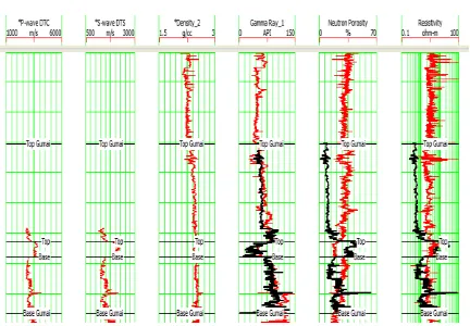
Figure 1. Available logs for the well X (from left to right: P-Wave, S-Wave, Density, Gamma ray, Neutron porosity, Resistivity)
Next was the data marker which was a boundary marker of a layer that becomes a zone of interest could be analogous as the top and base on a rock formation. Data marker was obtained from well report, in this research centered in gumai formation.
The second stage predicts 𝑣𝑠 was obtained from the Sonic log through the Castagna equation9 with the help of the Humpsell-Russhell 9 software as shown in figure 1. The basis of HRS-9 processing in the process log section used log transform equations 𝑣𝑠 that was generated by sonic logs. With the used of empirical relationships to predict 𝑣𝑠 had proven to be accurate but the usage must be accompanied by an effective medium for predictions 𝑣𝑠.10 Under the situation of lack of
share wave data, one method would be to predict a pseudo shear wave log from a measured compressional velocity by equation 1 called Castagna’s mudrock equation :
𝑣𝑠 = 0.862𝑣𝑝− 1.172 (1)
Basically the ideal input 𝑣𝑠 for rock physics analysis should be based on log measurement. This usually happens on old wells, but if there is no input 𝑣𝑠 from the log the wave should be predicted.
Based on lithostratigraphy11, the well X is
divided into four formations, namely Air Benakat at 0 - 605 m, Gumai at a depth of 605 m - 1165 m, Talang Akar at a depth of 1165 - 1504 m, Pre-Talang Akar at a depth of 1504 - 1750 m.12 This research is focused on Gumai
Formation because lithology in Gumai Formation is dominant flakes with sandstone inserts that are likely to find thin limestone inserts at the top. Figure 1 shows that the value response on each log that consists of P-Wave Log increases (>3000 m/s on a scale of 1000-6000 m/s), S-Wave Log increased (> 1750 m/s on a scale of 500-3000 m/s), Density Log stayed (> 2.25 g/cc on a scale of 1.5-3 g/cc), Gamma Ray log decreased (<75 API on a scale of 0-150 API), Neutron Porosity Log decreased (<35% scale 0-70%), Resistivity Log increased (> 50 ohm-m on a scale of 0.1-100 ohm-m).
From the analysis result, Gamma Ray response value to well in reservoir zone is seen decrease of Gamma Ray value indicating that the layer is non-shale. At the Density, Neutron Porosity, and resistivity values indicate that the rock layers are porous rocks and allow for hydrocarbon fillings, the reservoir zone is estimated to be at a depth between 922 m-980 m.
Figure 2. Ratio 𝑣𝑝to 𝑣𝑠 seen from Gamma Ray log.
The third stage, 𝑣𝑝 to 𝑣𝑠 cross-plot analysis intended to see anomalies that occurred in well X toward the changes in lithology and fluid.13 Figure 2 shows cross-plot between the ratio 𝑣𝑝/𝑣𝑠 represented in the Gamma Ray log, ranged between 27-39 API Units with an estimation S wave velocity 2000-2400 m/s and the approximate P Wave velocity 3400-3875 m/s in the red square refers to the following table 1.
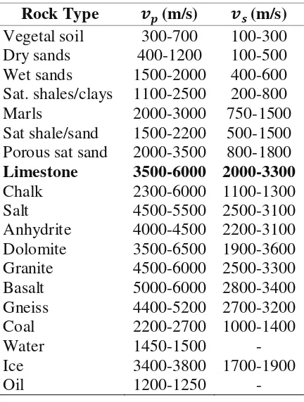
Table 1. Wave speeds of various rock types14 Rock Type 𝒗𝒑(m/s) 𝒗𝒔(m/s) Vegetal soil 300-700 100-300 Dry sands 400-1200 100-500 Wet sands 1500-2000 400-600 Sat. shales/clays 1100-2500 200-800 Marls 2000-3000 750-1500 Sat shale/sand 1500-2200 500-1500 Porous sat sand 2000-3500 800-1800 Limestone 3500-6000 2000-3300 Chalk 2300-6000 1100-1300 Salt 4500-5500 2500-3100 Anhydrite 4000-4500 2200-3100 Dolomite 3500-6500 1900-3600 Granite 4500-6000 2500-3300 Basalt 5000-6000 2800-3400 Gneiss 4400-5200 2700-3200 Coal 2200-2700 1000-1400 Water 1450-1500 - Ice 3400-3800 1700-1900
Oil 1200-1250 -
Table 1 shows that the speed of the 𝑣𝑝 and 𝑣𝑠, based on table 1, at well X with 𝑣𝑝 ranging
between 3500-6000 m/s and 𝑣𝑠 ranging from 2000 to 3300 m/s it belongs to the limestone rock category. It is also supported by geological well report that mention rock lithology exists in the research area is more dominant flakes with sandstone inserts, rocks and napal which are sometimes found thinly inserted limestones especially at the top. Gamma ray response was sensitive parameters to a change in rock lithology and able to differentiate shale and sand.
AVO was the interpretation angle to show that there was an increase or decrease in amplitude to offset. The basic assumption of AVO analysis was that seismic gathering is free from noise after preconditioning process data while maintaining amplitude response from data gather.
The Intercept A and Gradient B method is an approach to AVO which involves re-arranging the Aki-Richard equation to15
The Aki-Richard equation predicts a linear relationship between these amplitudes and
2 sin .
To understand the concept of AVO attribute, various approaches from the Zoeppritz theoretical equations, one of them that were used in this study was Shuey's two-term approximation.8
𝑅(𝜃) = 𝐴 + 𝐵𝑠𝑖𝑛2(𝜃) (3)
where R was the reflection coefficient, 𝜃 was the angle of incident, A was the AVO intercept and B was the AVO gradient.
Equation 3 was an amplitude function of the incident angle (𝜃). Intercept A represented the reflectivity of 𝑣𝑝 at zero angle and gradient B stated the amplitude change as a function of offset.
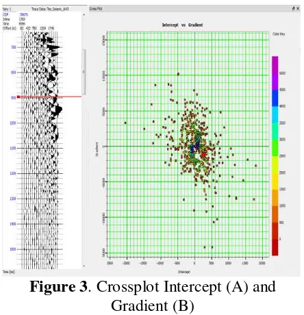
Figure 3. Crossplot Intercept (A) and Gradient (B)
Figure 3 was a crossplot in the lithologic zone that was indicated by sand and shale layers which was shown by supergather data of well X in time domain with red line and color key at value 0 indicated that intercept had positive value (+) and gradient had negative value (-).
Figure 4. Cross-section AVO in well X
Rutherford and William (1989) derived the following classification scheme for AVO anomalies, with the futher modifications by Ross and Kinman (1995) and Castagna (1997):
Class 1 : High acoustic impedance contrast Class 2 : Near-zero impedance contrast Class 2p : Same as 2, with polarity change Class 3 : Low impedance contrast
Class 4 : Very low impedance contrast Referring to the Rutherford-William AVO16 classification which states that grade 2 anomalies have near-zero acoustic contrast, sand in class 2 has an AI value similar to shale rocks often called dimspots or weak negative reflectors and has negative intercept and gradient values. In the target zone, it was generally equal to zero reflectivity depend on the value of the impedance and density. Second class AVO anomaly itself is divided into 2 kinds, negative intercept and negative gradient or 2p class which is anomaly with reversal of polarity and has positive intercept and negative gradient. Therefore, it can be concluded that the anomalies in the well X with positive intercept values (0.96-1) and the negative gradient (-0.96-(-1)) including AVO anomalies 2p class. Anomalies in the 2p class are usually found in drilling wells on the ground as they occur in areas of gas sandstone that have moderate to high rock compaction rates.
The dimspot case occurs in a reservoir that has a shale lithology composition, sand mixed with gas. The presence of gas mixture in sand litology will decrease the value of acoustic impedance characterized by reduced amplitude. The gas effect on the reservoir gives rise to positive polarity that will reduce the amplitude. Amplitude is zero which means there is no signal of reflection or it could also cause positive polarity.
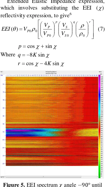
The fifth stage, determine best chi (𝜒) project angle for EEI analysis. Whitcombe et al. (2002) introduced Extended Elastic Impedance or EEI, they replaced the sin2 term in the two term Aki Richard equation with, to give the following expression for EEI reflectivity, REEI.17
Extended Elastic Impedance expression, which involves substituting the EEI () reflectivity expression, to give6
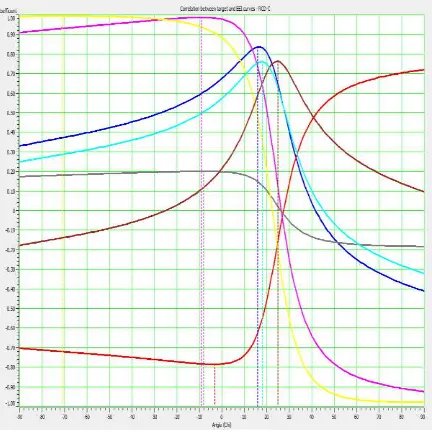
Figure 6. Correlation coefficients between target and EEI curves well X
In figure 6, the blue curve (density), the pink color (p-wave), the red color (volumetric), the black color (resistivity), the light blue (𝑠𝑤), the red color (NPHI), the yellow color (s-wave). For more detail the correlation coefficient is obtained for each log, is shown in the following table:
Table 2. Correlation result represents the maximum correlation of target logs and corresponding chi angle well X Target Log angle
(deg)
Correlation Coefficient (%)
Density 16 0.838497
P-Wave -9 0.989874
Volumetric 25 0.765313
Gamma Ray 25 0.83866
Resistivity -8 0.203301 Sw 18 0.810585
NPHI -3 0.782996 S-Wave -71 0.996658
Figure 7 illustrated the overlapping between the EEI log curve (black color) with the log well curve (red). From the value listed (EEI log unit was the impedance value) it was seen that the EEI curve showed good clarity in representing the target zone. As indicated by the correlation value in three log types (gamma ray, NPHI, resistivity).
Figure 7. Overlapping between Well Log and EEI Logs
EEI curves with 𝜒 angle gamma ray 25°, NPHI -3° dan resistivity -8° were able to assert the top and base of the target zone. These results indicated that EEI studies could be performed further using petrophysical analyzes that was derived through the EEI approach to a quantitative interpretation.
If at this stage the results which is obtained from overlapping well logs and EEI logs were not satisfactory, it was recommended to repeat from the beginning of the EEI angle determination.
From the result of 𝜒 angle dan koefisien korelasi pada semua log yang tersedia dengan range and correlation coefficient on all available logs with reasonable 𝜒 angle and the highest correlation coefficient was found in gamma ray 𝜒 angle 25° with correlation level 0.83866 on scale -1 until 1 (figure 8) to differentiate visually sand and shale lithology which if using AVO attribute analysis less clearly visible the difference.
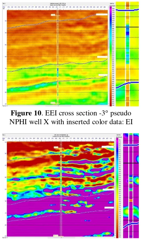
Figure 9. EEI cross section 25° pseudo gamma ray well X with inserted color data:
EI
Based on figure 9 the predicted top and base target zones impedance values was ranged from 7493-7765 (m/s)*(g/cc) with shale impedance between 7493-7551 (m/s)*(g/cc) and sand between 7571-7609 (m/s)*(g/cc). With a 25° 𝜒 angle capable of visually separating shale and sand lithology which in the AVO analysis had not been able to show significant differences.
Based on figure 10 the predicted top and base target zones impedance values was ranged from 5743-10625 (m/s)*(g/cc) with shale impedance between 8134-8831 (m/s)*(g/cc) and sand between 7038-7437 (m/s)*(g/cc). Assuming the impedance value implied that the value of the shale impedance was greater than the sand impedance value due to the geological conditions in the gumai formation of the research area there were flakes at the top of the formation.
Figure 10. EEI cross section -3° pseudo NPHI well X with inserted color data: EI
Figure 11. EEI cross section 16° pseudo density well X with inserted color data: EI
In this study the sand had a density lower than shale lithology, so the target inversion was to see a layer that had a low density. Based on figure 11 the predicted top and base target zone impedance values was ranged from 7046-7487 (m/s)*(g/cc) with shale impedance 7469-7487 (m/s)*(g/cc) and sand 7217-7397 (m/s)*(g/cc). The inversion analysis on pseudo density represented the possibility of low gas saturations in the study area, based on a sand impedance value lower than shale. With the mixing of gas in the sand lithology it would reduce the value of impedance.
Conclusions
922 m - 980 m with the top and the base in the formation of the gumai. For lithology based on geological data of tamper formation which tend to flakes, then it was used Greenberg-Castagna equation for mudrock. The selection of the equation should be based on the lithological conditions of the study area.
The AVO attribute analysis could show well dimensional anomalies, but in the case of sand and shale lithology identification still could not be illustrated visually sharply. From the AVO anomaly classification of the well X was categorized in the 2p class which was showed by the reversal of the polarity of positive intercept and negative gradient values. Furthermore, in EEI reflectivity analysis using 𝜒 angle 25° using gamma ray was able to describe visually sand and shale lithology that was looked almost the same.
References
1. Singh VB, Baid VK, Biswal S, Subrahmaniam D. Acoustic to Elastic Impedance – A New Tool for Reservoir Characterisation. 1998;(1374):1374–9. 2. Francis A, Hicks GJ. Porosity and Shale
Volume Estimation for the Ardmore Field Using Extended Elastic Impedance. Eage 68th Conf Exhib. 2006;(June 2006):1–5. 3. Fernandus A. Sandstone Reservoir
Characterization In Renax Fields with Extended Elastic Impedance Inversion. Bandung Institute of Technology; 2008. 4. Hadi JM. Extended Elastic Impedance
inversion for lithology and fluid identification review in Sandstone Gas Reservoir in Field North Sumatera Basin Walawala. Bandung Institute of Technology; 2009.
5. Woelandari D. The use of Extended Elastic Impedance Method for Separating Lithology and Fluid: A Case Study of
Carbonate Reservoirs in the field “X” in
the North West Java. University of Indonesia; 2010.
6. Shahri SG. Application of Extended Elastic Impedance (EEI) to improve Reservoir Characterization. 2013;(June). 7. Sismanto. Rock physics: Estimation
Approach Based Air Permeability and
Saturation Seismic Data. Yogyakarta: Graha Ilmu; 2013. 3-18 p.
8. Russell B. Extended Elastic Impedance using HRS-9.
9. Castagna JP, Batzle ML, Eastwood RL. Relationships between compressional‐ wave and shear‐ wave velocities in clastic silicate rocks. GEOPHYSICS. 1985 Apr;50(4):571–81.
10.Avseth P, Mukerji T, Mavko G. Quantitative Seismic Interpretation: Applying Rock Physics Tools to Reduce Interpretation Risk. Cambrigde University Press; 2005.
11.Sarjono, Sardjito. Hydrocarbon Source Rock Identification in the South Palembang Sub-Basin. In 1989. p. 427–66. 12. Exploration Department of Pertamina.
Well Report. Sumatera; 2000.
13. Lin J, Hsu S, Lin AT, Yeh Y, Lo C. Vp/Vs
distribution in the northern Taiwan area :
Implications for the tectonic structures and rock property variations. Tectonophysics. 2016;692:181–90.
14.Mavko G, Mukerji T, Dvorkin J. The Rock
Physics Handbook : Tools for Seismic
Analysis of Porous Media. Second. Stanford University, USA: Cambrigde University Press; 2009. 74 p.
15.Hosseini Shoar B, Javaherian A, Keshavarz Farajkhah N, Seddigh Arabani M. Reflectivity template, a quantitative intercept-gradient AVO analysis to study gas hydrate resources - A case study of Iranian deep sea sediments. Mar Pet Geol. 2014;51:184–96.
16.Rutherford SR, Williams RH. Amplitude‐ versus‐ offset variations in gas sands. GEOPHYSICS. 1989 Jun;54(6):680–8. 17. Russell BH, Lines LR, Hirsche KW, Peron