SPSS Advanced Statistics 17.0.pdf

(1)

i

(2)

Chicago, IL 60606-6412 Tel: (312) 651-3000 Fax: (312) 651-3668

SPSS is a registered trademark and the other product names are the trademarks of SPSS Inc. for its proprietary computer software. No material describing such software may be produced or distributed without the written permission of the owners of the trademark and license rights in the software and the copyrights in the published materials.

The SOFTWARE and documentation are provided with RESTRICTED RIGHTS. Use, duplication, or disclosure by the Government is subject to restrictions as set forth in subdivision (c) (1) (ii) of The Rights in Technical Data and Computer Software clause at 52.227-7013. Contractor/manufacturer is SPSS Inc., 233 South Wacker Drive, 11th Floor, Chicago, IL 60606-6412.

Patent No. 7,023,453

General notice: Other product names mentioned herein are used for identiﬁcation purposes only and may be trademarks of their respective companies.

Windows is a registered trademark of Microsoft Corporation.

Apple, Mac, and the Mac logo are trademarks of Apple Computer, Inc., registered in the U.S. and other countries.

Printed in the United States of America.

(3)

Preface

SPSS Statistics 17.0 is a comprehensive system for analyzing data. The Advanced Statistics optional add-on module provides the additional analytic techniques described in this manual. The Advanced Statistics add-on module must be used with the SPSS Statistics 17.0 Base system and is completely integrated into that system.

Installation

To install the Advanced Statistics add-on module, run the License Authorization Wizard using the authorization code that you received from SPSS Inc. For more information, see the installation instructions supplied with the Advanced Statistics add-on module.

Compatibility

SPSS Statistics is designed to run on many computer systems. See the installation instructions that came with your system for speciﬁc information on minimum and recommended requirements.

Serial Numbers

Your serial number is your identiﬁcation number with SPSS Inc. You will need this serial number when you contact SPSS Inc. for information regarding support, payment, or an upgraded system. The serial number was provided with your Base system.

Customer Service

If you have any questions concerning your shipment or account, contact your local ofﬁce, listed on the Web site athttp://www.spss.com/worldwide. Please have your serial number ready for identiﬁcation.

(4)

hands-on workshops. Seminars will be offered in major cities on a regular basis. For more information on these seminars, contact your local ofﬁce, listed on the Web site athttp://www.spss.com/worldwide.

Technical Support

Technical Support services are available to maintenance customers. Customers may contact Technical Support for assistance in using SPSS Statistics or for installation help for one of the supported hardware environments. To reach Technical Support, see the Web site athttp://www.spss.com, or contact your local ofﬁce, listed on the Web site athttp://www.spss.com/worldwide. Be prepared to identify yourself, your organization, and the serial number of your system.

Additional Publications

TheSPSS Statistical Procedures Companion, by Marija Norušis, has been published by Prentice Hall. A new version of this book, updated for SPSS Statistics 17.0, is planned. TheSPSS Advanced Statistical Procedures Companion, also based on SPSS Statistics 17.0, is forthcoming. TheSPSS Guide to Data Analysisfor SPSS Statistics 17.0 is also in development. Announcements of publications available exclusively through Prentice Hall will be available on the Web site at http://www.spss.com/estore(select your home country, and then clickBooks).

(5)

1 Introduction to Advanced Statistics

1

2 GLM Multivariate Analysis

3

GLM Multivariate Model . . . 6

Build Terms . . . 7

Sum of Squares . . . 7

GLM Multivariate Contrasts . . . 9

Contrast Types. . . 9

GLM Multivariate Profile Plots . . . 10

GLM Multivariate Post Hoc Comparisons . . . 12

GLM Save. . . 14

GLM Multivariate Options . . . 16

GLM Command Additional Features . . . 18

3 GLM Repeated Measures

19

GLM Repeated Measures Define Factors . . . 23

GLM Repeated Measures Model . . . 25

Build Terms . . . 26

GLM Repeated Measures Contrasts . . . 28

Contrast Types. . . 29

GLM Repeated Measures Profile Plots . . . 30

GLM Repeated Measures Post Hoc Comparisons . . . 31

GLM Repeated Measures Save. . . 34

(6)

4 Variance Components Analysis

39

Variance Components Model . . . 42

Variance Components Options . . . 43

Sum of Squares (Variance Components) . . . 44

Variance Components Save to New File . . . 46

VARCOMP Command Additional Features . . . 47

5 Linear Mixed Models

48

Linear Mixed Models Select Subjects/Repeated Variables . . . 51

Linear Mixed Models Fixed Effects . . . 53

Build Non-Nested Terms . . . 54

Build Nested Terms . . . 54

Linear Mixed Models Random Effects . . . 56

Linear Mixed Models Estimation . . . 58

Linear Mixed Models Statistics. . . 60

Linear Mixed Models EM Means . . . 62

Linear Mixed Models Save . . . 63

MIXED Command Additional Features. . . 64

(7)

6 Generalized Linear Models

65

Generalized Linear Models Response . . . 71

Generalized Linear Models Reference Category. . . 72

Generalized Linear Models Predictors . . . 74

Generalized Linear Models Options . . . 76

Generalized Linear Models Model . . . 77

Generalized Linear Models Estimation . . . 79

Generalized Linear Models Initial Values . . . 81

Generalized Linear Models Statistics . . . 83

Generalized Linear Models EM Means . . . 86

Generalized Linear Models Save. . . 88

Generalized Linear Models Export . . . 91

GENLIN Command Additional Features . . . 93

7 Generalized Estimating Equations

94

Generalized Estimating Equations Type of Model . . . 98

Generalized Estimating Equations Response . . . 103

Generalized Estimating Equations Reference Category . . . 105

Generalized Estimating Equations Predictors . . . 106

Generalized Estimating Equations Options . . . 108

Generalized Estimating Equations Model . . . 109

Generalized Estimating Equations Estimation . . . 111

Generalized Estimating Equations Initial Values . . . 113

Generalized Estimating Equations Statistics . . . 115

Generalized Estimating Equations EM Means . . . 118

Generalized Estimating Equations Save. . . 121

(8)

8 Model Selection Loglinear Analysis

126

Loglinear Analysis Define Range. . . 128

Loglinear Analysis Model . . . 129

Model Selection Loglinear Analysis Options . . . 130

HILOGLINEAR Command Additional Features . . . 131

9 General Loglinear Analysis

132

General Loglinear Analysis Model . . . 135

General Loglinear Analysis Options. . . 136

General Loglinear Analysis Save. . . 137

GENLOG Command Additional Features . . . 138

10 Logit Loglinear Analysis

139

Logit Loglinear Analysis Model . . . 142

Logit Loglinear Analysis Options . . . 144

Logit Loglinear Analysis Save . . . 145

GENLOG Command Additional Features . . . 146

(9)

11 Life Tables

147

Life Tables Define Events for Status Variables . . . 150

Life Tables Define Range. . . 150

Life Tables Options . . . 151

SURVIVAL Command Additional Features . . . 152

12 Kaplan-Meier Survival Analysis

153

Kaplan-Meier Define Event for Status Variable . . . 155

Kaplan-Meier Compare Factor Levels . . . 156

Kaplan-Meier Save New Variables . . . 157

Kaplan-Meier Options. . . 158

KM Command Additional Features . . . 158

13 Cox Regression Analysis

160

Cox Regression Define Categorical Variables . . . 162

Cox Regression Plots . . . 164

Cox Regression Save New Variables. . . 165

Cox Regression Options . . . 166

Cox Regression Define Event for Status Variable. . . 167

COXREG Command Additional Features . . . 167

(10)

Computing a Time-Dependent Covariate . . . 169

Cox Regression with Time-Dependent Covariates Additional Features . 170

Appendices

A Categorical Variable Coding Schemes

171

Deviation . . . 171

Simple . . . 172

Helmert . . . 173

Difference . . . 173

Polynomial . . . 174

Repeated . . . 175

Special . . . 176

Indicator. . . 177

B Covariance Structures

178 Index

183

(11)

Chapter

1

Introduction to Advanced

Statistics

The Advanced Statistics option provides procedures that offer more advanced modeling options than are available through the Base system.

GLM Multivariate extends the general linear model provided by GLM Univariate to allow multiple dependent variables. A further extension, GLM Repeated Measures, allows repeated measurements of multiple dependent variables.

Variance Components Analysis is a speciﬁc tool for decomposing the variability in a dependent variable intoﬁxed and random components.

Linear Mixed Models expands the general linear model so that the data are permitted to exhibit correlated and nonconstant variability. The mixed linear model, therefore, provides theﬂexibility of modeling not only the means of the data but the variances and covariances as well.

Generalized Linear Models (GZLM) relaxes the assumption of normality for the error term and requires only that the dependent variable be linearly related to the predictors through a transformation, or link function. Generalized Estimating Equations (GEE) extends GZLM to allow repeated measurements.

General Loglinear Analysis allows you toﬁt models for cross-classiﬁed count data, and Model Selection Loglinear Analysis can help you to choose between models.

Logit Loglinear Analysis allows you toﬁt loglinear models for analyzing the relationship between a categorical dependent and one or more categorical predictors.

Survival analysis is available through Life Tables for examining the distribution of time-to-event variables, possibly by levels of a factor variable; Kaplan-Meier Survival Analysis for examining the distribution of time-to-event variables, possibly by levels of a factor variable or producing separate analyses by levels of a

(12)

(13)

Chapter

2

GLM Multivariate Analysis

The GLM Multivariate procedure provides regression analysis and analysis of variance for multiple dependent variables by one or more factor variables or covariates. The factor variables divide the population into groups. Using this general linear model procedure, you can test null hypotheses about the effects of factor variables on the means of various groupings of a joint distribution of dependent variables. You can investigate interactions between factors as well as the effects of individual factors. In addition, the effects of covariates and covariate interactions with factors can be included. For regression analysis, the independent (predictor) variables are speciﬁed as covariates.

Both balanced and unbalanced models can be tested. A design is balanced if each cell in the model contains the same number of cases. In a multivariate model, the sums of squares due to the effects in the model and error sums of squares are in matrix form rather than the scalar form found in univariate analysis. These matrices are called SSCP (sums-of-squares and cross-products) matrices. If more than one dependent variable is speciﬁed, the multivariate analysis of variance using Pillai’s trace, Wilks’ lambda, Hotelling’s trace, and Roy’s largest root criterion with approximateFstatistic are provided as well as the univariate analysis of variance for each dependent variable. In addition to testing hypotheses, GLM Multivariate produces estimates of parameters.

Commonly useda prioricontrasts are available to perform hypothesis testing. Additionally, after an overallFtest has shown significance, you can use post hoc tests to evaluate differences among specific means. Estimated marginal means give estimates of predicted mean values for the cells in the model, and profile plots (interaction plots) of these means allow you to visualize some of the relationships easily. The post hoc multiple comparison tests are performed for each dependent variable separately.

Residuals, predicted values, Cook’s distance, and leverage values can be saved as new variables in your dataﬁle for checking assumptions. Also available are a residual SSCP matrix, which is a square matrix of sums of squares and cross-products of residuals, a residual covariance matrix, which is the residual SSCP matrix divided

(14)

by the degrees of freedom of the residuals, and the residual correlation matrix, which is the standardized form of the residual covariance matrix.

WLS Weight allows you to specify a variable used to give observations different weights for a weighted least-squares (WLS) analysis, perhaps to compensate for different precision of measurement.

Example. A manufacturer of plastics measures three properties of plasticfilm: tear resistance, gloss, and opacity. Two rates of extrusion and two different amounts of additive are tried, and the three properties are measured under each combination of extrusion rate and additive amount. The manufacturerfinds that the extrusion rate and the amount of additive individually produce significant results but that the interaction of the two factors is not significant.

Methods. Type I, Type II, Type III, and Type IV sums of squares can be used to evaluate different hypotheses. Type III is the default.

Statistics. Post hoc range tests and multiple comparisons: least signiﬁcant difference, Bonferroni, Sidak, Scheffé, Ryan-Einot-Gabriel-Welsch multipleF, Ryan-Einot-Gabriel-Welsch multiple range, Student-Newman-Keuls, Tukey’s honestly signiﬁcant difference, Tukey’sb, Duncan, Hochberg’s GT2, Gabriel, Waller Duncant test, Dunnett (one-sided and two-sided), Tamhane’s T2, Dunnett’s T3, Games-Howell, and Dunnett’sC. Descriptive statistics: observed means, standard deviations, and counts for all of the dependent variables in all cells; the Levene test for homogeneity of variance; Box’sMtest of the homogeneity of the covariance matrices of the dependent variables; and Bartlett’s test of sphericity.

Plots. Spread-versus-level, residual, and proﬁle (interaction).

Data.The dependent variables should be quantitative. Factors are categorical and can have numeric values or string values. Covariates are quantitative variables that are related to the dependent variable.

(15)

5

GLM Multivariate Analysis

Related procedures. Use the Explore procedure to examine the data before doing an analysis of variance. For a single dependent variable, use GLM Univariate. If you measured the same dependent variables on several occasions for each subject, use GLM Repeated Measures.

Obtaining GLM Multivariate Tables

E _{From the menus choose:}

Analyze

General Linear Model Multivariate...

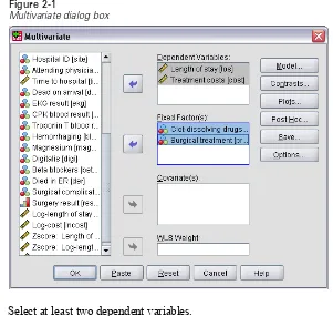
Figure 2-1

Multivariate dialog box

E Select at least two dependent variables.

(16)

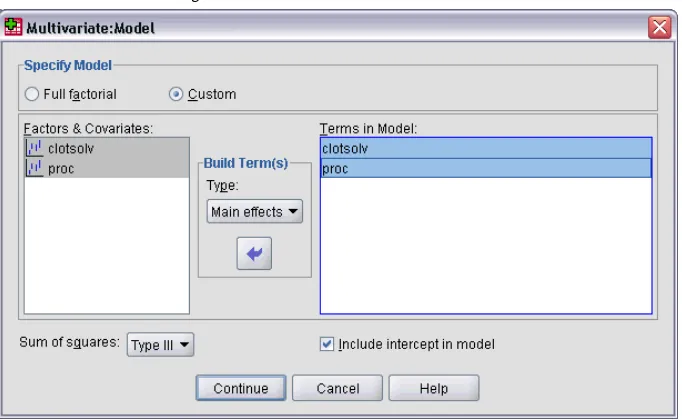
GLM Multivariate Model

Figure 2-2

Multivariate Model dialog box

Specify Model.A full factorial model contains all factor main effects, all covariate main effects, and all factor-by-factor interactions. It does not contain covariate interactions. SelectCustomto specify only a subset of interactions or to specify factor-by-covariate interactions. You must indicate all of the terms to be included in the model.

Factors and Covariates.The factors and covariates are listed.

Model.The model depends on the nature of your data. After selectingCustom, you can select the main effects and interactions that are of interest in your analysis.

Sum of squares. The method of calculating the sums of squares. For balanced or unbalanced models with no missing cells, the Type III sum-of-squares method is most commonly used.

(17)

7

Build Terms

For the selected factors and covariates:

Interaction.Creates the highest-level interaction term of all selected variables. This is the default.

Main effects.Creates a main-effects term for each variable selected.

All 2-way.Creates all possible two-way interactions of the selected variables.

All 3-way.Creates all possible three-way interactions of the selected variables.

All 4-way.Creates all possible four-way interactions of the selected variables.

All 5-way.Creates all possibleﬁve-way interactions of the selected variables.

Sum of Squares

For the model, you can choose a type of sums of squares. Type III is the most commonly used and is the default.

Type I.This method is also known as the hierarchical decomposition of the

sum-of-squares method. Each term is adjusted for only the term that precedes it in the model. Type I sums of squares are commonly used for:

A balanced ANOVA model in which any main effects are specified before any first-order interaction effects, anyfirst-order interaction effects are specified before any second-order interaction effects, and so on.

A polynomial regression model in which any lower-order terms are speciﬁed before any higher-order terms.

A purely nested model in which thefirst-specified effect is nested within the second-specified effect, the second-specified effect is nested within the third, and so on. (This form of nesting can be specified only by using syntax.)

Type II.This method calculates the sums of squares of an effect in the model adjusted for all other “appropriate” effects. An appropriate effect is one that corresponds to all effects that do not contain the effect being examined. The Type II sum-of-squares method is commonly used for:

A balanced ANOVA model.

(18)

Any regression model.

A purely nested design. (This form of nesting can be speciﬁed by using syntax.) Type III.The default. This method calculates the sums of squares of an effect in the design as the sums of squares adjusted for any other effects that do not contain it and orthogonal to any effects (if any) that contain it. The Type III sums of squares have one major advantage in that they are invariant with respect to the cell frequencies as long as the general form of estimability remains constant. Hence, this type of sums of squares is often considered useful for an unbalanced model with no missing cells. In a factorial design with no missing cells, this method is equivalent to the Yates’ weighted-squares-of-means technique. The Type III sum-of-squares method is commonly used for:

Any models listed in Type I and Type II.

Any balanced or unbalanced model with no empty cells.

Type IV.This method is designed for a situation in which there are missing cells. For any effectFin the design, ifFis not contained in any other effect, then Type IV = Type III = Type II. WhenFis contained in other effects, Type IV distributes the contrasts being made among the parameters inFto all higher-level effects equitably. The Type IV sum-of-squares method is commonly used for:

(19)

9

GLM Multivariate Contrasts

Figure 2-3

Multivariate Contrasts dialog box

Contrasts are used to test whether the levels of an effect are signiﬁcantly different from one another. You can specify a contrast for each factor in the model. Contrasts represent linear combinations of the parameters.

Hypothesis testing is based on the null hypothesisLBM = 0, whereLis the contrast coefﬁcients matrix,Mis the identity matrix (which has dimension equal to the number of dependent variables), andBis the parameter vector. When a contrast is speciﬁed, anLmatrix is created such that the columns corresponding to the factor match the contrast. The remaining columns are adjusted so that theLmatrix is estimable.

In addition to the univariate test usingFstatistics and the Bonferroni-type simultaneous conﬁdence intervals based on Student’stdistribution for the contrast differences across all dependent variables, the multivariate tests using Pillai’s trace, Wilks’ lambda, Hotelling’s trace, and Roy’s largest root criteria are provided.

Available contrasts are deviation, simple, difference, Helmert, repeated, and polynomial. For deviation contrasts and simple contrasts, you can choose whether the reference category is the last orﬁrst category.

Contrast Types

(20)

Simple. Compares the mean of each level to the mean of a speciﬁed level. This type of contrast is useful when there is a control group. You can choose theﬁrst or last category as the reference.

Difference.Compares the mean of each level (except theﬁrst) to the mean of previous levels. (Sometimes called reverse Helmert contrasts.)

Helmert.Compares the mean of each level of the factor (except the last) to the mean of subsequent levels.

Repeated. Compares the mean of each level (except the last) to the mean of the subsequent level.

Polynomial. Compares the linear effect, quadratic effect, cubic effect, and so on. The ﬁrst degree of freedom contains the linear effect across all categories; the second degree of freedom, the quadratic effect; and so on. These contrasts are often used to estimate polynomial trends.

GLM Multivariate Profile Plots

Figure 2-4

(21)

11

Profile plots (interaction plots) are useful for comparing marginal means in your model. A profile plot is a line plot in which each point indicates the estimated marginal mean of a dependent variable (adjusted for any covariates) at one level of a factor. The levels of a second factor can be used to make separate lines. Each level in a third factor can be used to create a separate plot. All factors are available for plots. Profile plots are created for each dependent variable.

A proﬁle plot of one factor shows whether the estimated marginal means are increasing or decreasing across levels. For two or more factors, parallel lines indicate that there is no interaction between factors, which means that you can investigate the levels of only one factor. Nonparallel lines indicate an interaction.

Figure 2-5

Nonparallel plot (left) and parallel plot (right)

(22)

GLM Multivariate Post Hoc Comparisons

Figure 2-6

Multivariate Post Hoc Multiple Comparisons for Observed Means dialog box

Post hoc multiple comparison tests. Once you have determined that differences exist among the means, post hoc range tests and pairwise multiple comparisons can determine which means differ. Comparisons are made on unadjusted values. The post hoc tests are performed for each dependent variable separately.

(23)

13

Hochberg’s GT2is similar to Tukey’s honestly signiﬁcant difference test, but the Studentized maximum modulus is used. Usually, Tukey’s test is more powerful. Gabriel’s pairwise comparisons testalso uses the Studentized maximum modulus and is generally more powerful than Hochberg’s GT2 when the cell sizes are unequal. Gabriel’s test may become liberal when the cell sizes vary greatly.

Dunnett’s pairwise multiple comparison t testcompares a set of treatments against a single control mean. The last category is the default control category. Alternatively, you can choose theﬁrst category. You can also choose a two-sided or one-sided test. To test that the mean at any level (except the control category) of the factor is not equal to that of the control category, use a two-sided test. To test whether the mean at any level of the factor is smaller than that of the control category, select< Control. Likewise, to test whether the mean at any level of the factor is larger than that of the control category, select> Control.

Ryan, Einot, Gabriel, and Welsch (R-E-G-W) developed two multiple step-down range tests. Multiple step-down proceduresﬁrst test whether all means are equal. If all means are not equal, subsets of means are tested for equality.R-E-G-W Fis based on anFtest andR-E-G-W Qis based on the Studentized range. These tests are more powerful than Duncan’s multiple range test and Student-Newman-Keuls (which are also multiple step-down procedures), but they are not recommended for unequal cell sizes.

When the variances are unequal, useTamhane’s T2(conservative pairwise comparisons test based on attest),Dunnett’s T3(pairwise comparison test based on the Studentized maximum modulus),Games-Howell pairwise comparison test(sometimes liberal), orDunnett’s C(pairwise comparison test based on the Studentized range).

Duncan’s multiple range test, Student-Newman-Keuls (S-N-K), andTukey’s b are range tests that rank group means and compute a range value. These tests are not used as frequently as the tests previously discussed.

TheWaller-Duncan t testuses a Bayesian approach. This range test uses the harmonic mean of the sample size when the sample sizes are unequal.

(24)

The least signiﬁcant difference (LSD) pairwise multiple comparison test is equivalent to multiple individualttests between all pairs of groups. The disadvantage of this test is that no attempt is made to adjust the observed signiﬁcance level for multiple comparisons.

Tests displayed. Pairwise comparisons are provided for LSD, Sidak, Bonferroni, Games-Howell, Tamhane’s T2 and T3, Dunnett’sC, and Dunnett’s T3. Homogeneous subsets for range tests are provided for S-N-K, Tukey’sb, Duncan, R-E-G-WF, R-E-G-WQ, and Waller. Tukey’s honestly signiﬁcant difference test, Hochberg’s GT2, Gabriel’s test, and Scheffé’s test are both multiple comparison tests and range tests.

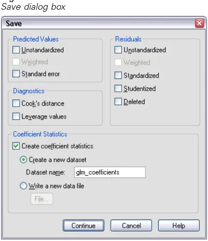
GLM Save

Figure 2-7 Save dialog box

You can save values predicted by the model, residuals, and related measures as new variables in the Data Editor. Many of these variables can be used for examining assumptions about the data. To save the values for use in another SPSS Statistics session, you must save the current dataﬁle.

(25)

15

Unstandardized.The value the model predicts for the dependent variable.

Weighted.Weighted unstandardized predicted values. Available only if a WLS variable was previously selected.

Standard error.An estimate of the standard deviation of the average value of the dependent variable for cases that have the same values of the independent variables.

Diagnostics.Measures to identify cases with unusual combinations of values for the independent variables and cases that may have a large impact on the model.

Cook's distance.A measure of how much the residuals of all cases would change if a particular case were excluded from the calculation of the regression coefﬁcients. A large Cook's D indicates that excluding a case from computation of the regression statistics changes the coefﬁcients substantially.

Leverage values.Uncentered leverage values. The relative inﬂuence of each observation on the model'sﬁt.

Residuals. An unstandardized residual is the actual value of the dependent variable minus the value predicted by the model. Standardized, Studentized, and deleted residuals are also available. If a WLS variable was chosen, weighted unstandardized residuals are available.

Unstandardized.The difference between an observed value and the value predicted by the model.

Weighted.Weighted unstandardized residuals. Available only if a WLS variable was previously selected.

Standardized. The residual divided by an estimate of its standard deviation. Standardized residuals, which are also known as Pearson residuals, have a mean of 0 and a standard deviation of 1.

Studentized.The residual divided by an estimate of its standard deviation that varies from case to case, depending on the distance of each case's values on the independent variables from the means of the independent variables.

Deleted.The residual for a case when that case is excluded from the calculation of the regression coefﬁcients. It is the difference between the value of the dependent variable and the adjusted predicted value.

(26)

row of significance values for thetstatistics corresponding to the parameter estimates, and a row of residual degrees of freedom. For a multivariate model, there are similar rows for each dependent variable. You can use this matrixfile in other procedures that read matrixfiles.

GLM Multivariate Options

Figure 2-8

Multivariate Options dialog box

(27)

17

Estimated Marginal Means. Select the factors and interactions for which you want estimates of the population marginal means in the cells. These means are adjusted for the covariates, if any. Interactions are available only if you have speciﬁed a custom model.

Compare main effects. Provides uncorrected pairwise comparisons among

estimated marginal means for any main effect in the model, for both between- and within-subjects factors. This item is available only if main effects are selected under the Display Means For list.

Confidence interval adjustment. Select least signiﬁcant difference (LSD),

Bonferroni, or Sidak adjustment to the conﬁdence intervals and signiﬁcance. This item is available only ifCompare main effectsis selected.

Display.SelectDescriptive statisticsto produce observed means, standard deviations, and counts for all of the dependent variables in all cells.Estimates of effect sizegives a partial eta-squared value for each effect and each parameter estimate. The eta-squared statistic describes the proportion of total variability attributable to a factor. Select Observed powerto obtain the power of the test when the alternative hypothesis is set based on the observed value. SelectParameter estimatesto produce the parameter estimates, standard errors,ttests, conﬁdence intervals, and the observed power for each test. You can display the hypothesis and errorSSCP matricesand theResidual SSCP matrixplus Bartlett’s test of sphericity of the residual covariance matrix.

(28)

Significance level. You might want to adjust the significance level used in post hoc tests and the confidence level used for constructing confidence intervals. The specified value is also used to calculate the observed power for the test. When you specify a significance level, the associated level of the confidence intervals is displayed in the dialog box.

GLM Command Additional Features

These features may apply to univariate, multivariate, or repeated measures analysis. The command syntax language also allows you to:

Specify nested effects in the design (using theDESIGNsubcommand).

Specify tests of effects versus a linear combination of effects or a value (using theTESTsubcommand).

Specify multiple contrasts (using theCONTRASTsubcommand).

Include user-missing values (using theMISSINGsubcommand).

Specify EPS criteria (using theCRITERIAsubcommand).

Construct a customLmatrix,Mmatrix, orKmatrix (using theLMATRIX, MMATRIX, orKMATRIXsubcommands).

For deviation or simple contrasts, specify an intermediate reference category (using theCONTRASTsubcommand).

Specify metrics for polynomial contrasts (using theCONTRASTsubcommand).

Specify error terms for post hoc comparisons (using thePOSTHOCsubcommand).

Compute estimated marginal means for any factor or factor interaction among the factors in the factor list (using theEMMEANSsubcommand).

Specify names for temporary variables (using theSAVEsubcommand).

Construct a correlation matrix dataﬁle (using theOUTFILEsubcommand). Construct a matrix dataﬁle that contains statistics from the between-subjects

ANOVA table (using theOUTFILEsubcommand).

(29)

Chapter

3

GLM Repeated Measures

The GLM Repeated Measures procedure provides analysis of variance when the same measurement is made several times on each subject or case. If between-subjects factors are speciﬁed, they divide the population into groups. Using this general linear model procedure, you can test null hypotheses about the effects of both the between-subjects factors and the within-subjects factors. You can investigate interactions between factors as well as the effects of individual factors. In addition, the effects of constant covariates and covariate interactions with the between-subjects factors can be included.

In a doubly multivariate repeated measures design, the dependent variables represent measurements of more than one variable for the different levels of the within-subjects factors. For example, you could have measured both pulse and respiration at three different times on each subject.

The GLM Repeated Measures procedure provides both univariate and multivariate analyses for the repeated measures data. Both balanced and unbalanced models can be tested. A design is balanced if each cell in the model contains the same number of cases. In a multivariate model, the sums of squares due to the effects in the model and error sums of squares are in matrix form rather than the scalar form found in univariate analysis. These matrices are called SSCP (sums-of-squares and cross-products) matrices. In addition to testing hypotheses, GLM Repeated Measures produces estimates of parameters.

Commonly useda prioricontrasts are available to perform hypothesis testing on between-subjects factors. Additionally, after an overallFtest has shown significance, you can use post hoc tests to evaluate differences among specific means. Estimated marginal means give estimates of predicted mean values for the cells in the model, and profile plots (interaction plots) of these means allow you to visualize some of the relationships easily.

Residuals, predicted values, Cook’s distance, and leverage values can be saved as new variables in your dataﬁle for checking assumptions. Also available are a residual SSCP matrix, which is a square matrix of sums of squares and cross-products of residuals, a residual covariance matrix, which is the residual SSCP matrix divided

(30)

by the degrees of freedom of the residuals, and the residual correlation matrix, which is the standardized form of the residual covariance matrix.

WLS Weight allows you to specify a variable used to give observations different weights for a weighted least-squares (WLS) analysis, perhaps to compensate for different precision of measurement.

Example.Twelve students are assigned to a high- or low-anxiety group based on their scores on an anxiety-rating test. The anxiety rating is called a between-subjects factor because it divides the subjects into groups. The students are each given four trials on a learning task, and the number of errors for each trial is recorded. The errors for each trial are recorded in separate variables, and a within-subjects factor (trial) is defined with four levels for the four trials. The trial effect is found to be significant, while the trial-by-anxiety interaction is not significant.

Methods. Type I, Type II, Type III, and Type IV sums of squares can be used to evaluate different hypotheses. Type III is the default.

Statistics.Post hoc range tests and multiple comparisons (for between-subjects factors): least signiﬁcant difference, Bonferroni, Sidak, Scheffé, Ryan-Einot-Gabriel-Welsch multipleF, Ryan-Einot-Gabriel-Welsch multiple range, Student-Newman-Keuls, Tukey’s honestly signiﬁcant difference, Tukey’sb, Duncan, Hochberg’s GT2, Gabriel, Waller Duncanttest, Dunnett (one-sided and two-sided), Tamhane’s T2, Dunnett’s T3, Games-Howell, and Dunnett’sC. Descriptive statistics: observed means, standard deviations, and counts for all of the dependent variables in all cells; the Levene test for homogeneity of variance; Box’sM; and Mauchly’s test of sphericity.

Plots. Spread-versus-level, residual, and proﬁle (interaction).

Data. The dependent variables should be quantitative. Between-subjects factors divide the sample into discrete subgroups, such as male and female. These factors are categorical and can have numeric values or string values. Within-subjects factors are deﬁned in the Repeated Measures Deﬁne Factor(s) dialog box. Covariates are quantitative variables that are related to the dependent variable. For a repeated measures analysis, these should remain constant at each level of a within-subjects variable.

(31)

21

GLM Repeated Measures

taken on different days. If measurements of the same property were taken onfive days, the within-subjects factor could be specified asdaywithfive levels.

For multiple within-subjects factors, the number of measurements for each subject is equal to the product of the number of levels of each factor. For example, if measurements were taken at three different times each day for four days, the total number of measurements is 12 for each subject. The within-subjects factors could be speciﬁed asday(4)andtime(3).

Assumptions.A repeated measures analysis can be approached in two ways, univariate and multivariate.

The univariate approach (also known as the split-plot or mixed-model approach) considers the dependent variables as responses to the levels of within-subjects factors. The measurements on a subject should be a sample from a multivariate normal distribution, and the variance-covariance matrices are the same across the cells formed by the between-subjects effects. Certain assumptions are made on the variance-covariance matrix of the dependent variables. The validity of theFstatistic used in the univariate approach can be assured if the variance-covariance matrix is circular in form (Huynh and Mandeville, 1979).

To test this assumption, Mauchly’s test of sphericity can be used, which performs a test of sphericity on the variance-covariance matrix of an orthonormalized transformed dependent variable. Mauchly’s test is automatically displayed for a repeated measures analysis. For small sample sizes, this test is not very powerful. For large sample sizes, the test may be significant even when the impact of the departure on the results is small. If the significance of the test is large, the hypothesis of sphericity can be assumed. However, if the significance is small and the sphericity assumption appears to be violated, an adjustment to the numerator and denominator degrees of freedom can be made in order to validate the univariateFstatistic. Three estimates of this adjustment, which is calledepsilon, are available in the GLM Repeated Measures procedure. Both the numerator and denominator degrees of freedom must be multiplied by epsilon, and the significance of theFratio must be evaluated with the new degrees of freedom.

The multivariate approach considers the measurements on a subject to be a sample from a multivariate normal distribution, and the variance-covariance matrices are the same across the cells formed by the between-subjects effects. To test whether the variance-covariance matrices across the cells are the same, Box’sMtest can be used.

(32)

(for example, pre-test and post-test) and there are no between-subjects factors, you can use the Paired-Samples T Test procedure.

Obtaining GLM Repeated Measures

Analyze

General Linear Model Repeated Measures...

Figure 3-1

Repeated Measures Define Factor(s) dialog box

E _{Type a within-subject factor name and its number of levels.}

E _Click_Add_.

E _{Repeat these steps for each within-subjects factor.}

To deﬁne measure factors for a doubly multivariate repeated measures design:

(33)

23

E _Click_Add_.

After deﬁning all of your factors and measures:

E _Click_Define_.

Figure 3-2

Repeated Measures dialog box

E _{Select a dependent variable that corresponds to each combination of within-subjects}

factors (and optionally, measures) on the list.

To change positions of the variables, use the up and down arrows.

To make changes to the within-subjects factors, you can reopen the Repeated Measures Deﬁne Factor(s) dialog box without closing the main dialog box. Optionally, you can specify between-subjects factor(s) and covariates.

GLM Repeated Measures Define Factors

(34)

p. 22. Note that the order in which you specify within-subjects factors is important. Each factor constitutes a level within the previous factor.

To use Repeated Measures, you must set up your data correctly. You must deﬁne within-subjects factors in this dialog box. Notice that these factors are not existing variables in your data but rather factors that you deﬁne here.

Example.In a weight-loss study, suppose the weights of several people are measured each week forfive weeks. In the datafile, each person is a subject or case. The weights for the weeks are recorded in the variablesweight1,weight2, and so on. The gender of each person is recorded in another variable. The weights, measured for each subject repeatedly, can be grouped by defining a within-subjects factor. The factor could be calledweek, defined to havefive levels. In the main dialog box, the variablesweight1, ...,weight5are used to assign thefive levels ofweek. The variable in the datafile that groups males and females (gender) can be specified as a between-subjects factor to study the differences between males and females.

(35)

25

GLM Repeated Measures Model

Figure 3-3

Repeated Measures Model dialog box

Between-Subjects. The between-subjects factors and covariates are listed.

(36)

Sum of squares.The method of calculating the sums of squares for the between-subjects model. For balanced or unbalanced between-subjects models with no missing cells, the Type III sum-of-squares method is the most commonly used.

Build Terms

Sum of Squares

For the model, you can choose a type of sums of squares. Type III is the most commonly used and is the default.

sum-of-squares method. Each term is adjusted for only the term that precedes it in the model. Type I sums of squares are commonly used for:

(37)

27

Type II.This method calculates the sums of squares of an effect in the model adjusted for all other “appropriate” effects. An appropriate effect is one that corresponds to all effects that do not contain the effect being examined. The Type II sum-of-squares method is commonly used for:

A balanced ANOVA model.

Any model that has main factor effects only.

Any regression model.

A purely nested design. (This form of nesting can be speciﬁed by using syntax.)

Type III.The default. This method calculates the sums of squares of an effect in the design as the sums of squares adjusted for any other effects that do not contain it and orthogonal to any effects (if any) that contain it. The Type III sums of squares have one major advantage in that they are invariant with respect to the cell frequencies as long as the general form of estimability remains constant. Hence, this type of sums of squares is often considered useful for an unbalanced model with no missing cells. In a factorial design with no missing cells, this method is equivalent to the Yates’ weighted-squares-of-means technique. The Type III sum-of-squares method is commonly used for:

Any balanced or unbalanced model with no empty cells.

Type IV.This method is designed for a situation in which there are missing cells. For any effectFin the design, ifFis not contained in any other effect, then Type IV = Type III = Type II. WhenFis contained in other effects, Type IV distributes the contrasts being made among the parameters inFto all higher-level effects equitably. The Type IV sum-of-squares method is commonly used for:

(38)

GLM Repeated Measures Contrasts

Figure 3-4

Repeated Measures Contrasts dialog box

Contrasts are used to test for differences among the levels of a between-subjects factor. You can specify a contrast for each between-subjects factor in the model. Contrasts represent linear combinations of the parameters.

Hypothesis testing is based on the null hypothesisLBM=0, whereLis the contrast coefﬁcients matrix,Bis the parameter vector, andMis the average matrix that corresponds to the average transformation for the dependent variable. You can display this transformation matrix by selectingTransformation matrixin the Repeated Measures Options dialog box. For example, if there are four dependent variables, a within-subjects factor of four levels, and polynomial contrasts (the default) are used for within-subjects factors, theMmatrix will be (0.5 0.5 0.5 0.5)’. When a contrast is speciﬁed, anLmatrix is created such that the columns corresponding to the between-subjects factor match the contrast. The remaining columns are adjusted so that theLmatrix is estimable.

Available contrasts are deviation, simple, difference, Helmert, repeated, and polynomial. For deviation contrasts and simple contrasts, you can choose whether the reference category is the last orﬁrst category.

(39)

29

Contrast Types

Deviation.Compares the mean of each level (except a reference category) to the mean of all of the levels (grand mean). The levels of the factor can be in any order.

Simple. Compares the mean of each level to the mean of a speciﬁed level. This type of contrast is useful when there is a control group. You can choose theﬁrst or last category as the reference.

Difference.Compares the mean of each level (except theﬁrst) to the mean of previous levels. (Sometimes called reverse Helmert contrasts.)

Helmert.Compares the mean of each level of the factor (except the last) to the mean of subsequent levels.

Repeated. Compares the mean of each level (except the last) to the mean of the subsequent level.

(40)

GLM Repeated Measures Profile Plots

Figure 3-5

Repeated Measures Profile Plots dialog box

Profile plots (interaction plots) are useful for comparing marginal means in your model. A profile plot is a line plot in which each point indicates the estimated marginal mean of a dependent variable (adjusted for any covariates) at one level of a factor. The levels of a second factor can be used to make separate lines. Each level in a third factor can be used to create a separate plot. All factors are available for plots. Profile plots are created for each dependent variable. Both between-subjects factors and within-subjects factors can be used in profile plots.

(41)

31

Figure 3-6

Nonparallel plot (left) and parallel plot (right)

After a plot is speciﬁed by selecting factors for the horizontal axis and, optionally, factors for separate lines and separate plots, the plot must be added to the Plots list.

GLM Repeated Measures Post Hoc Comparisons

Figure 3-7

(42)

Post hoc multiple comparison tests. Once you have determined that differences exist among the means, post hoc range tests and pairwise multiple comparisons can determine which means differ. Comparisons are made on unadjusted values. These tests are not available if there are no between-subjects factors, and the post hoc multiple comparison tests are performed for the average across the levels of the within-subjects factors.

The Bonferroni and Tukey’s honestly significant difference tests are commonly used multiple comparison tests. TheBonferroni test, based on Student’ststatistic, adjusts the observed significance level for the fact that multiple comparisons are made. Sidak’s t testalso adjusts the significance level and provides tighter bounds than the Bonferroni test. Tukey’s honestly significant difference testuses the Studentized range statistic to make all pairwise comparisons between groups and sets the experimentwise error rate to the error rate for the collection for all pairwise comparisons. When testing a large number of pairs of means, Tukey’s honestly significant difference test is more powerful than the Bonferroni test. For a small number of pairs, Bonferroni is more powerful.

Hochberg’s GT2is similar to Tukey’s honestly signiﬁcant difference test, but the Studentized maximum modulus is used. Usually, Tukey’s test is more powerful. Gabriel’s pairwise comparisons testalso uses the Studentized maximum modulus and is generally more powerful than Hochberg’s GT2 when the cell sizes are unequal. Gabriel’s test may become liberal when the cell sizes vary greatly.

Dunnett’s pairwise multiple comparison t testcompares a set of treatments against a single control mean. The last category is the default control category. Alternatively, you can choose theﬁrst category. You can also choose a two-sided or one-sided test. To test that the mean at any level (except the control category) of the factor is not equal to that of the control category, use a two-sided test. To test whether the mean at any level of the factor is smaller than that of the control category, select< Control. Likewise, to test whether the mean at any level of the factor is larger than that of the control category, select> Control.

(43)

33

When the variances are unequal, useTamhane’s T2(conservative pairwise comparisons test based on attest),Dunnett’s T3(pairwise comparison test based on the Studentized maximum modulus),Games-Howell pairwise comparison test(sometimes liberal), orDunnett’s C(pairwise comparison test based on the Studentized range).

Duncan’s multiple range test, Student-Newman-Keuls (S-N-K), andTukey’s b are range tests that rank group means and compute a range value. These tests are not used as frequently as the tests previously discussed.

TheWaller-Duncan t testuses a Bayesian approach. This range test uses the harmonic mean of the sample size when the sample sizes are unequal.

The signiﬁcance level of theScheffétest is designed to allow all possible linear combinations of group means to be tested, not just pairwise comparisons available in this feature. The result is that the Scheffé test is often more conservative than other tests, which means that a larger difference between means is required for signiﬁcance.

The least signiﬁcant difference (LSD) pairwise multiple comparison test is equivalent to multiple individualttests between all pairs of groups. The disadvantage of this test is that no attempt is made to adjust the observed signiﬁcance level for multiple comparisons.

(44)

GLM Repeated Measures Save

Figure 3-8

Repeated Measures Save dialog box

You can save values predicted by the model, residuals, and related measures as new variables in the Data Editor. Many of these variables can be used for examining assumptions about the data. To save the values for use in another SPSS Statistics session, you must save the current dataﬁle.

Predicted Values.The values that the model predicts for each case.

Unstandardized.The value the model predicts for the dependent variable.

Standard error.An estimate of the standard deviation of the average value of the dependent variable for cases that have the same values of the independent variables.

(45)

35

Cook's distance.A measure of how much the residuals of all cases would change if a particular case were excluded from the calculation of the regression coefﬁcients. A large Cook's D indicates that excluding a case from computation of the regression statistics changes the coefﬁcients substantially.

Leverage values.Uncentered leverage values. The relative inﬂuence of each observation on the model'sﬁt.

Residuals. An unstandardized residual is the actual value of the dependent variable minus the value predicted by the model. Standardized, Studentized, and deleted residuals are also available.

Unstandardized.The difference between an observed value and the value predicted by the model.

Standardized. The residual divided by an estimate of its standard deviation. Standardized residuals, which are also known as Pearson residuals, have a mean of 0 and a standard deviation of 1.

Studentized.The residual divided by an estimate of its standard deviation that varies from case to case, depending on the distance of each case's values on the independent variables from the means of the independent variables.

Deleted.The residual for a case when that case is excluded from the calculation of the regression coefﬁcients. It is the difference between the value of the dependent variable and the adjusted predicted value.

(46)

GLM Repeated Measures Options

Figure 3-9

Repeated Measures Options dialog box

Optional statistics are available from this dialog box. Statistics are calculated using a ﬁxed-effects model.

(47)

37

Compare main effects. Provides uncorrected pairwise comparisons among

estimated marginal means for any main effect in the model, for both between- and within-subjects factors. This item is available only if main effects are selected under the Display Means For list.

Confidence interval adjustment. Select least signiﬁcant difference (LSD),

Bonferroni, or Sidak adjustment to the conﬁdence intervals and signiﬁcance. This item is available only ifCompare main effectsis selected.

Display.SelectDescriptive statisticsto produce observed means, standard deviations, and counts for all of the dependent variables in all cells.Estimates of effect sizegives a partial eta-squared value for each effect and each parameter estimate. The eta-squared statistic describes the proportion of total variability attributable to a factor. Select Observed powerto obtain the power of the test when the alternative hypothesis is set based on the observed value. SelectParameter estimatesto produce the parameter estimates, standard errors,ttests, conﬁdence intervals, and the observed power for each test. You can display the hypothesis and errorSSCP matricesand theResidual SSCP matrixplus Bartlett’s test of sphericity of the residual covariance matrix.

Homogeneity testsproduces the Levene test of the homogeneity of variance for each dependent variable across all level combinations of the between-subjects factors, for between-subjects factors only. Also, homogeneity tests include Box’sMtest of the homogeneity of the covariance matrices of the dependent variables across all level combinations of the between-subjects factors. The spread-versus-level and residual plots options are useful for checking assumptions about the data. This item is disabled if there are no factors. SelectResidual plotsto produce an observed-by-predicted-by-standardized residuals plot for each dependent variable. These plots are useful for investigating the assumption of equal variance. Select Lack of fit testto check if the relationship between the dependent variable and the independent variables can be adequately described by the model. General estimable functionallows you to construct custom hypothesis tests based on the general estimable function. Rows in any contrast coefﬁcient matrix are linear combinations of the general estimable function.

(48)

GLM Command Additional Features

These features may apply to univariate, multivariate, or repeated measures analysis. The command syntax language also allows you to:

Specify tests of effects versus a linear combination of effects or a value (using theTESTsubcommand).

Specify multiple contrasts (using theCONTRASTsubcommand).

Construct a customLmatrix,Mmatrix, orKmatrix (using theLMATRIX, MMATRIX, andKMATRIXsubcommands).

For deviation or simple contrasts, specify an intermediate reference category (using theCONTRASTsubcommand).

Specify metrics for polynomial contrasts (using theCONTRASTsubcommand). Specify error terms for post hoc comparisons (using thePOSTHOCsubcommand).

Compute estimated marginal means for any factor or factor interaction among the factors in the factor list (using theEMMEANSsubcommand).

Specify names for temporary variables (using theSAVEsubcommand).

Construct a correlation matrix dataﬁle (using theOUTFILEsubcommand). Construct a matrix dataﬁle that contains statistics from the between-subjects

ANOVA table (using theOUTFILEsubcommand).

(49)

Chapter

4

Variance Components Analysis

The Variance Components procedure, for mixed-effects models, estimates the contribution of each random effect to the variance of the dependent variable. This procedure is particularly interesting for analysis of mixed models such as split plot, univariate repeated measures, and random block designs. By calculating variance components, you can determine where to focus attention in order to reduce the variance.

Four different methods are available for estimating the variance components: minimum norm quadratic unbiased estimator (MINQUE), analysis of variance (ANOVA), maximum likelihood (ML), and restricted maximum likelihood (REML). Various speciﬁcations are available for the different methods.

Default output for all methods includes variance component estimates. If the ML method or the REML method is used, an asymptotic covariance matrix table is also displayed. Other available output includes an ANOVA table and expected mean squares for the ANOVA method and an iteration history for the ML and REML methods. The Variance Components procedure is fully compatible with the GLM Univariate procedure.

WLS Weight allows you to specify a variable used to give observations different weights for a weighted analysis, perhaps to compensate for variations in precision of measurement.

Example. At an agriculture school, weight gains for pigs in six different litters are measured after one month. The litter variable is a random factor with six levels. (The six litters studied are a random sample from a large population of pig litters.) The investigatorﬁnds out that the variance in weight gain is attributable to the difference in litters much more than to the difference in pigs within a litter.

Data.The dependent variable is quantitative. Factors are categorical. They can have numeric values or string values of up to eight bytes. At least one of the factors must be random. That is, the levels of the factor must be a random sample of possible levels. Covariates are quantitative variables that are related to the dependent variable.

(50)

Assumptions.All methods assume that model parameters of a random effect have zero means andﬁnite constant variances and are mutually uncorrelated. Model parameters from different random effects are also uncorrelated.

The residual term also has a zero mean andﬁnite constant variance. It is uncorrelated with model parameters of any random effect. Residual terms from different observations are assumed to be uncorrelated.

Based on these assumptions, observations from the same level of a random factor are correlated. This fact distinguishes a variance component model from a general linear model.

ANOVA and MINQUE do not require normality assumptions. They are both robust to moderate departures from the normality assumption.

ML and REML require the model parameter and the residual term to be normally distributed.

Related procedures. Use the Explore procedure to examine the data before doing variance components analysis. For hypothesis testing, use GLM Univariate, GLM Multivariate, and GLM Repeated Measures.

Obtaining Variance Components Tables

Analyze

(51)

41

Variance Components Analysis

Figure 4-1

Variance Components dialog box

E _{Select a dependent variable.}

E _{Select variables for Fixed Factor(s), Random Factor(s), and Covariate(s), as appropriate}

(52)

Variance Components Model

Figure 4-2

Variance Components Model dialog box

Factors & Covariates. The factors and covariates are listed.

Model.The model depends on the nature of your data. After selectingCustom, you can select the main effects and interactions that are of interest in your analysis. The model must contain a random factor.

(53)

43

Build Terms

Variance Components Options

Figure 4-3

Variance Components Options dialog box

(54)

MINQUE(minimum norm quadratic unbiased estimator) produces estimates that are invariant with respect to theﬁxed effects. If the data are normally distributed and the estimates are correct, this method produces the least variance among all unbiased estimators. You can choose a method for random-effect prior weights.

ANOVA(analysis of variance) computes unbiased estimates using either the Type I or Type III sums of squares for each effect. The ANOVA method sometimes produces negative variance estimates, which can indicate an incorrect model, an inappropriate estimation method, or a need for more data.

Maximum likelihood(ML) produces estimates that would be most consistent with the data actually observed, using iterations. These estimates can be biased. This method is asymptotically normal. ML and REML estimates are invariant under translation. This method does not take into account the degrees of freedom used to estimate theﬁxed effects.

Restricted maximum likelihood(REML) estimates reduce the ANOVA estimates for many (if not all) cases of balanced data. Because this method is adjusted for the ﬁxed effects, it should have smaller standard errors than the ML method. This method takes into account the degrees of freedom used to estimate theﬁxed effects.

Random Effect Priors.Uniformimplies that all random effects and the residual term have an equal impact on the observations. TheZeroscheme is equivalent to assuming zero random-effect variances. Available only for the MINQUE method.

Sum of Squares.Type Isums of squares are used for the hierarchical model, which is often used in variance component literature. If you chooseType III, the default in GLM, the variance estimates can be used in GLM Univariate for hypothesis testing with Type III sums of squares. Available only for the ANOVA method.

Criteria. You can specify the convergence criterion and the maximum number of iterations. Available only for the ML or REML methods.

Display. For the ANOVA method, you can choose to display sums of squares and expected mean squares. If you selectedMaximum likelihoodorRestricted maximum likelihood, you can display a history of the iterations.

Sum of Squares (Variance Components)

(55)

45

sum-of-squares method. Each term is adjusted for only the term that precedes it in the model. The Type I sum-of-squares method is commonly used for:

A purely nested model in which thefirst-specified effect is nested within the second-specified effect, the second-specified effect is nested within the third, and so on. (This form of nesting can be specified only by using syntax.)

Type III.The default. This method calculates the sums of squares of an effect in the design as the sums of squares adjusted for any other effects that do not contain it and orthogonal to any effects (if any) that contain it. The Type III sums of squares have one major advantage in that they are invariant with respect to the cell frequencies as long as the general form of estimability remains constant. Therefore, this type is often considered useful for an unbalanced model with no missing cells. In a factorial design with no missing cells, this method is equivalent to the Yates’ weighted-squares-of-means technique. The Type III sum-of-squares method is commonly used for:

Any models listed in Type I.

(56)

Variance Components Save to New File

Figure 4-4

Variance Components Save to New File dialog box

You can save some results of this procedure to a new SPSS Statistics datafile. Variance component estimates. Saves estimates of the variance components and estimate labels to a datafile or dataset. These can be used in calculating more statistics or in further analysis in the GLM procedures. For example, you can use them to calculate confidence intervals or test hypotheses.

Component covariation.Saves a variance-covariance matrix or a correlation matrix to a dataﬁle or dataset. Available only ifMaximum likelihoodorRestricted maximum likelihoodhas been speciﬁed.

Destination for created values. Allows you to specify a dataset name or external filename for thefile containing the variance component estimates and/or the matrix. Datasets are available for subsequent use in the same session but are not saved asfiles unless explicitly saved prior to the end of the session. Dataset names must conform to variable naming rules.

(57)

47

VARCOMP Command Additional Features

The command syntax language also allows you to:

SPSS Advanced Statistics 17.0.pdf

i

Preface

Contents

1

Introduction to Advanced Statistics

1

2

GLM Multivariate Analysis

3

3

GLM Repeated Measures

19

4

Variance Components Analysis

39

5

Linear Mixed Models

48

6

Generalized Linear Models

65

7

Generalized Estimating Equations

94

8

Model Selection Loglinear Analysis

126

9

General Loglinear Analysis

132

10 Logit Loglinear Analysis

139

11 Life Tables

147

12 Kaplan-Meier Survival Analysis

153

13 Cox Regression Analysis

160

Appendices

A Categorical Variable Coding Schemes

171

B Covariance Structures

178

Index

183

Chapter

1

Introduction to Advanced

Statistics

Chapter

2

GLM Multivariate Analysis

GLM Multivariate Model

Build Terms

Sum of Squares

GLM Multivariate Contrasts

Contrast Types

GLM Multivariate Profile Plots

GLM Multivariate Post Hoc Comparisons

GLM Save

GLM Multivariate Options

GLM Command Additional Features

Chapter

3

GLM Repeated Measures

GLM Repeated Measures Define Factors

GLM Repeated Measures Model

Build Terms

Sum of Squares

GLM Repeated Measures Contrasts

Contrast Types

GLM Repeated Measures Profile Plots

GLM Repeated Measures Post Hoc Comparisons

GLM Repeated Measures Save

GLM Repeated Measures Options

GLM Command Additional Features

Chapter

4

Variance Components Analysis