Fundamentals of Evolutionary Game Theory and its Applications pdf pdf

(1)

(2)

Volume 6

Evolutionary Economics and Social Complexity

Science

Editors-in-Chief

Takahiro Fujimoto and Yuji Aruka

The Japanese Association for Evolutionary Economics (JAFEE) always has adhered to its original aim of taking an explicit “integrated” approach. This path has been followed steadfastly since the Association’s establishment in 1997 and, as well, since the inauguration of our international journal in 2004. We have deployed an agenda encompassing a contemporary array of subjects including but not limited to: foundations of institutional and evolutionary economics, criticism of mainstream views in the social sciences, knowledge and learning in socio-economic life, development and innovation of technologies, transformation of industrial organizations and economic systems, experimental studies in economics, agentbased modeling of socio-economic systems, evolution of the governance structure of firms and other organizations, comparison of dynamically changing institutions of the world, and policy proposals in the transformational process of economic life. In short, our starting point is an “integrative science” of evolutionary and institutional views. Furthermore,we always endeavor to stay abreast of newly established methods such as agent-based modeling, socio/econo-physics, and network analysis as part of our integrative links.

More fundamentally, “evolution” in social science is interpreted as an essential key word, i.e., an integrative and/or communicative link to understand and re-domain various preceding dichotomies in the sciences: ontological or epistemological, subjective or objective, homogeneous or heterogeneous, natural or artificial, selfish or altruistic, individualistic or collective, rational or irrational, axiomatic or psychological-based, causal nexus or cyclic networked, optimal or adaptive, microor

macroscopic, deterministic or stochastic, historical or theoretical, mathematical or computational, experimental or empirical, agent-based or socio/econo-physical, institutional or evolutionary,

regional or global, and so on. The conventional meanings adhering to various traditional dichotomies may be more or less obsolete, to be replaced with more current ones vis-à-vis contemporary

(3)

implementing new ideas. We thus are keen to look for “integrated principles” common to the above-mentioned dichotomies throughout our serial compilation of publications.We are also encouraged to create a new, broader spectrum for establishing a specific method positively integrated in our own original way.

(4)

Jun Tanimoto

Fundamentals of Evolutionary Game Theory and

its Applications

(5)

Jun Tanimoto

Graduate School of Engineering Sciences, Kyushu University Interdisciplinary, Fukuoka, Fukuoka, Japan

ISSN 2198-4204 e-ISSN 2198-4212

ISBN 978-4-431-54961-1 e-ISBN 978-4-431-54962-8 DOI 10.1007/978-4-431-54962-8

Springer Tokyo Heidelberg New York Dordrecht London

Library of Congress Control Number: 2015951623 © Springer Japan 2015

This work is subject to copyright. All rights are reserved by the Publisher, whether the whole or part of the material is concerned, specifically the rights of translation, reprinting, reuse of illustrations, recitation, broadcasting, reproduction on microfilms or in any other physical way, and transmission or information storage and retrieval, electronic adaptation, computer software, or by similar or dissimilar methodology now known or hereafter developed.

The use of general descriptive names, registered names, trademarks, service marks, etc. in this publication does not imply, even in the absence of a specific statement, that such names are exempt from the relevant protective laws and regulations and therefore free for general use.

The publisher, the authors and the editors are safe to assume that the advice and information in this book are believed to be true and accurate at the date of publication. Neither the publisher nor the authors or the editors give a warranty, express or implied, with respect to the material contained herein or for any errors or omissions that may have been made.

Printed on acid-free paper

(6)

Preface

For more than 25 years, I have been studying environmental issues that affect humans, human societies, and the living environment. I started my research career by studying building physics; in particular, I was concerned with hygrothermal transfer problems in building envelopes and

predictions of thermal loads. After my Ph.D. work, I extended my research field to a special scale

perspective. This extension was motivated by several factors. One was that I noticed a reciprocal influence between an individual building environment and the entire urban environment. Another was that the so-called urban heat island problem began to draw much attention in the 1990s. Mitigation of urban heating contributes to energy conservation and helps improve urban amenity; hence, the urban heat island problem became one of the most prominent social issues of the time. Thus, I started to study urban climatology because I was mainly concerned with why and how an urban heat island forms. The problem was approached with sophisticated tools, such as wind tunnel experiments, field observations, and computational fluid dynamics (CFD), and was backed by deep theories concerning heat transfer and fluid dynamics. A series of such studies forced me to realize that to obtain

meaningful and reasonable solutions, we should focus not only on one area (e.g., the scale of building physics) but also on several neighboring areas that involve complex feedback interactions (e.g.,

scales of urban canopies and of urban climatology). It is crucially important to establish new bridges that connect several areas having different spatiotemporal scales.

This experience made me realize another crucial point. The term “environment” encompasses a very wide range of objects: nature, man-made physical systems, society, and humanity itself. One obvious fact is that we cannot achieve any significant progress in solving so-called environmental problems as long as we focus on just a single issue; everything is profoundly interdependent. Turning on an air conditioner is not the final solution for feeling comfortable. The operation of an air

conditioner increases urban air temperatures; therefore, the efficiency of the overall system inevitably goes down and more energy must be provided to the system. This realization might deter someone from using an air conditioner. This situation is one intelligible example. The decisions of any

individual human affect the environment, and the decisions of a society as a collection of individuals may substantially impact the environment. In turn, the environment reacts to those decisions made by individuals and society, and some of that feedback is likely to be negative. Such feedback crucially influences our decision-making processes. Interconnected cycling systems always work in this way.

With this realization, I recognized the concept of a combined human–environmental–social system. To reach the crux of the environmental problem, which includes physical mechanisms, individual humans, and society, we must study the combination of these diverse phenomena as an integrated environmental system. We must consider all interactions between these different systems at all scales.

I know well that this is easy to say and not so easy to do. I recognize the difficulties in attempting to establish a new bridge that connects several fields governed by completely different principles, such as natural environmental systems and human systems. I understand that I stand before a steep mountain path.

(7)

making, and a thorough understanding of decision making is essential to build that new bridge. Thus, for the last decade, I have been deeply committed to the study of evolutionary game theory and

statistical physics.

This book shares the knowledge I have gained so far in collaboration with graduate students and other researchers who are interested in evolutionary game theory and its applications. It will be a great pleasure for me if this book can give readers some insight into recent progress and some hints as to how we should proceed.

(8)

Acknowledgments

This book owes its greatest debt to my coworkers who had been my excellent students. Chapter 2

relies at critical points on the contributions of Dr. Hiroki Sagara (Panasonic Factory Solutions Co. Ltd.) and Mr. Satoshi Kokubo (Mitsubishi Electric Corporation). Dr. Atsuo Yamauchi (Meidensha Corporation), Mr. Satoshi Kokubo, Mr. Keizo Shigaki (Rico Co. Ltd.), Mr. Takashi Ogasawara (Mitsubishi Electric Corporation), and Ms. Eriko Fukuda (Ph.D. candidate at Kyushu University) gave very substantial input to the content of Chap. 3 . Chapter 5 would not have been completed without the many new findings of Dr. Atsuo Yamauchi, Mr. Makoto Nakata (SCSK Corporation), Mr. Shinji Kukida (Toshiba Corporation), Mr. Kezo Shigaki, and Mr. Takuya Fujiki (Toyota Motor

Corporation) based on the new concept that traffic flow analysis can be dovetailed with evolutionary game theory. Chapter 6 is the product of dedicated effort by Ms. Eriko Fukuda in seeking another interesting challenge that can be addressed with evolutionary game theory. I sincerely express my gratitude to these people as well as to Dr. Zheng Wang (JSPS [Japan Society for the Promotion of Science] Fellow at Kyushu University) who works with our group, is regarded as one of the keenest young scholars, and deals with game and complex network theory. Continuous discussions with all these collaborators have helped me advance our studies and realize much satisfaction from our efforts.

(9)

Biography of the Author

Jun Tanimoto

was born in 1965 in Fukuoka, but he grew up in Yokohama. He graduated in 1988 from the Department of Architecture, Undergraduate School of Science & Engineering, at Waseda University. In 1990, he completed his master’s degree, and in 1993, he earned his doctoral degree from Waseda. He started his professional career as a research associate at Tokyo

Metropolitan University in 1990, moved to Kyushu University and was promoted to assistant professor (senior lecturer) in 1995, and became an associate professor in 1998. Since 2003, he has served as professor and head of the Laboratory of Urban Architectural Environmental Engineering. He was a visiting professor at the National Renewable Energy Laboratory (NREL), USA; at the University of New South Wales, Australia; and at

Eindhoven University of Technology, the Netherlands. Professor Tanimoto has published numerous scientific papers in building physics, urban climatology, and statistical physics and is the author of books including Mathematical Analysis of Environmental System (Springer; ISBN: 978-4-431-54621-4). He was a recipient of the Award of the Society of Heating, Air-Conditioning, and Sanitary Engineers of Japan (SHASE), the Fosterage Award from the Architectural Institute of Japan (AIJ), the Award of AIJ, and the IEEE CEC2009 Best Paper Award. He is involved in numerous activities worldwide, including being an editor of several international journals including PLOS One and the

Journal of Building Performance Simulation , among others; a committee member at many conferences; and an expert at the IEA Solar Heating and Cooling Program Task 23. He is also an active painter and novelist, and has been awarded numerous prizes in fine art and literature. He has created many works of art and published several books. He specializes in scenic drawing with

(14)

(1)

Jun Tanimoto, Fundamentals of Evolutionary Game Theory and its Applications, Evolutionary Economics and Social Complexity Science 6, DOI 10.1007/978-4-431-54962-8_1

1. Human–Environment–Social System and

Evolutionary Game Theory

Jun Tanimoto

1

Abstract

In this chapter, we discuss both the definition of an environmental system as one of the typical

dynamical systems and its relation to evolutionary game theory. We also outline the structure of each chapter in this book.

1.1 Modeling a Real Complex World

We define the word “system” as a collection of elements, all of which are connected organically to form an aggregate of elements that collectively possess an overall function. We know that most real systems are not time constant but time variable, i.e., they are “dynamical system s.” According to the common sense of the fields of science and engineering, a dynamical system can be described by space and time variables, i.e., x and t. Therefore, a dynamical system has a spatiotemporal structure.

Any system in the real world looks very complex. An environmental system is a typical example. If an environmental system is interpreted literally, considering every system involved with the

environment, we can see there is a lot of variety within it.

This variety arises from interactions between different environments (e.g., natural, human, and social) and differences in spatial scale (i.e., from the microscopic world weaved by microorganisms to the global environment as a whole, see Fig. 1.1). To reach the crux of an environmental problem, we must observe and consider diverse phenomena together, as an integrated environmental system, considering all interactions between the different systems and scales (Fig. 1.1). Accordingly, we have coined the phrase “human–environmental–social system” to encompass all these diverse

(15)

Fig. 1.1 Wide range of spatial scales over which environmental systems act, and the concept of the human–environmental–social system (Tanimoto 2014)

One important aspect that is revealed when you shed some light on the human–environment–social system is that human intention and behavior, either supported by rational decision making, in some cases, or irrational decision making, in others, has a crucial impact on its dynamics. In fact, what is called “global warming,” as one example of a global environmental problem, can be understood because of human overconsumption of fossil fuels over the course of the past couple of centuries, which seems rational for people only concerned with current comfort but seems irrational for people who are carefully considering long-term consequences. Hence, in seeking to establish a certain

provision to improve environmental problems, one needs to consider complex interactions between physical environmental systems and humans as well as social systems as a holistic system of

(16)

1.2 Evolutionary Game Theory

Why do we cooperate? Why do we observe many animals cooperating? The mysterious labyrinth surrounding how cooperative behavior can emerge in the real world has attracted much attention. The classical metaphor for investigating this social problem is the prisoner’s dilemma (PD ) game, which has been thought most appropriate, and is most frequently used as a template for social dilemma.

Evolutionary game theory (e.g. Weibull 1995) has evolved from game theory by merging it with the basic concept of Darwinism so as to compensate for the idea of time evolution, which is partially lacking in the original game theory that primarily deals with equilibrium.

Game theory was established in the mid-twentieth century by a novel contribution by von

Neumann and Morgenstern (von Neumann and Morgenstern 1944). After the inception they provided, the biggest milestone in driving the theory forward and making it more applicable to various fields (not only economics but also biology, information science, statistical physics, and other social sciences) was provided by John Nash, one of the three game theorists awarded the Nobel Prize. He did this by forming the equilibrium concept, known as Nash Equilibrium (Nash 1949). Another important contribution to evolutionary game theory was provided, in the 1980s, by Maynard Smith (Maynard Smith 1982). He formulated a central concept of evolutionary game theory called the evolutionarily stable strategy. In the 1990s, with the rapid growth of computational capabilities,

multi-agent simulation started to strongly drive evolutionary game theory, allowing one to easily build a flexible model, free from the premises that previous theoretical frameworks presumed.1_This

enables game players in these models to behave more intelligently and realistically. Consequently, many people have been attracted to seeking answers for the question of why we can observe so much evidence of the reciprocity mechanism working in real human social systems, and also among animal species, even during encounters with severe social dilemma situations, in which the theory predicts that game players should act defectively. As one example, the theory shows that all players would be trapped as complete defectors in the case of PD , which will be explained later in this book.

However, we can observe a lot of evidence that opposes this in the real world, where we ourselves and even some animal spices show social harmony with mutual cooperation in the respective social context (Fig. 1.2).

Fig. 1.2 How are humans able to establish reciprocity when encountering a social dilemma situation in the real world?

Since these developments, thousands of papers have been produced on research performed by means of computer simulations. Most of them follow the same pattern, in which each of the new

models they build a priori is shown with numerical results indicating more enhanced cooperation than what the theory predicts. Those are meaningful from the constructivism viewpoint, but still less

(17)

Nowak successfully made progress in understanding this problem, to some extent, with his

ground-breaking research (Nowak 2006). He proved theoretically that all the reciprocity mechanisms that bring mutual cooperation can be classified into four types, and all of them, amazingly, have

similar inequality conditions for evolving cooperation due to the so-called Hamilton Rule. Nowak calls all these fundamental mechanisms “social viscosity .” The Hamilton Rule (Hamilton 1964) finally solved the puzzle, which was originally posed by Charles Darwin’s book—The Origin of Species (1859)—of why sterile social insects, such as honey bees, leave reproduction to their sisters by arguing that a selection benefit to related organisms would allow the evolution of a trait that

confers the benefit but destroys the individual at the same time. Hamilton clearly deduced that kin selection favors cooperative behavior as long as the inclusive fitness surge due to the concept of relatedness is larger than the dilemma strength. This finding by Nowak, though he assumed several premises in his analytical procedure, elucidates that all the reciprocity mechanisms ever discussed can be explained with a simple mathematical formula, very similar to the Hamilton Rule, implying that “Nature is controlled by a simple rule.” The Nowak classifications—kin selection, direct

reciprocity , indirect reciprocity , network reciprocity , and group selection —successfully presented a new level to the controversy, but there have still been a lot of papers reporting “how much

cooperation thrives if you rely on our particular model”-type stories, because Nowak’s deduction is based on several limitations, and thus the real reciprocity mechanism may differ from it. In fact, among the five mechanisms, network reciprocity has been very well received, since people believe complex social networks may relate to emerging mutual cooperation in social system.

This is why this book primarily focuses network reciprocity in Chap. 3.

1.3 Structure of This Book

This book does not try to cover all the developments concerning evolutionary games, not even all the most important ones. In fact, it strives to describe several fundamental issues, a selected set of core elements of both evolutionary games and network reciprocity , and self-contained applications, which are drawn from our studies over the last decade.

Chapter 2 describes some theoretical foundations for dealing with evolutionary games in view of so-called social dilemma games. Some points such as universal scaling for dilemma strength might be useful from a theoretical viewpoint.

In Chap. 3, we focus on network reciprocity . We provide a transparent discussion on why limiting game opponents with a network helps the emergence of cooperation.

The remaining chapters demonstrate real-life applications of evolutionary games. Chapter 4

touches on the story of what triggers evolving communication among animal species. Chapter 5

demonstrates that social dilemma seems ubiquitous, even in traffic flow, which has been thought to be one of the typical applications that fluid dynamics deals with. Chapter 6 concerns spreading

epidemics and social provision for this by vaccination through the vaccination game, one of the hottest areas in evolutionary games.

References

(18)

1

Maynard Smith, J. 1982. Evolution and the theory of games. Cambridge: Cambridge University Press. [MATH][CrossRef]

Nash, J.F. 1949. Equilibrium points in n-person games. Proceedings of the National Academy of Science of the United States of America 36(1): 48–49.

[MathSciNet][CrossRef][ADS]

Nowak, M.A. 2006. Five rules for the evolution of cooperation. Science 314: 1560–1563. [PubMedCentral][CrossRef][PubMed][ADS]

Tanimoto, J. 2014. Mathematical analysis of environmental system. Tokyo: Springer. [MATH][CrossRef]

Von Neumann, J., and O. Morgenstern. 1944. Theory of games and economic behavior. Princeton: Princeton University Press. [MATH]

Weibull, J.W. 1995. Evolutionary game theory. Cambridge: MIT Press. [MATH]

Footnotes

(19)

(1)

Jun Tanimoto, Fundamentals of Evolutionary Game Theory and its Applications, Evolutionary Economics and Social Complexity Science 6, DOI 10.1007/978-4-431-54962-8_2

2. Fundamental Theory for Evolutionary Games

Jun Tanimoto

1

Abstract

In this chapter, we take a look at the appropriate treatment of linear dynamical systems, which you may be familiar with if you have taken some standard engineering undergraduate classes. The discussion is then extended to non-linear systems and their general dynamic properties. In this discussion, we introduce the 2-player and 2-strategy (2 × 2) game, which is the most important archetype among evolutionary games. Multi-player and 2-strategy games are also introduced. In the latter parts of this chapter, we define the dilemma strength, which is useful for the universal

comparison of the various reciprocity mechanisms supported by different models.

2.1 Linear Dynamical Systems

Let us start with an example. Consider the dynamics of an arbitrary linear thermal system.1_One

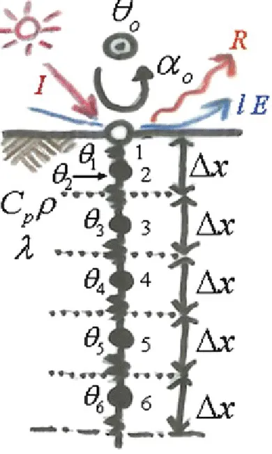
typical case is a thermal field of semi-infinite soil, as shown in Fig. 2.1. The x-coordinate axis takes the ground surface as its origin and measures depth underground. Underground heat propagates only by conduction, but convective heat transfer occurs on the ground surface, which is exposed to the external temperature. Also, radiation, evaporative cooling, and incoming solar radiation have an effect on the surface. As can be seen in Fig. 2.1, a discretization of space has been imposed, and thus the system is no longer continuous. The system featured, with thermal mass M, is affected by thermal conduction, convection, liberalized radiation, evaporative cooling, and solar radiation. Therefore, the temperature field is variable with time (t). All thermal balance equations, located on nodes

(20)

Fig. 2.1 Space discretization model based on Control Volume Method in which the surface layers of the semi-infinite soil are lumped parameterized

(2.1) Here, θ is a vector of unknown variables, which is each temperature of the nodes of the underground. M is called the heat capacitance matrix. C is called the heat conductance matrix, and the vector– matrix product Cθ expresses the influence of heat conduction. Another vector–matrix product C _oθ _o means the influence derived from heat convection. The vector f indicates other thermal influences given by a form of heat flux. Thermal influences other than conduction happening with in the system, expressed by , are called boundary condition. One extremely important thing is that the

system state equation has universal form. Regardless of what particular problem you have, as long as linear system it would be, what you see as a final equation is always same as expressed in Eq. (2.1). It might be understood by the fact that Eq. (2.1) can be likened to the Newton’s equation of motion for a particle, where implies first derivation of velocity; namely acceleration, M is literally “mass”, and the terms appeared in the right side; imply respective forces acting on the particle.

By the concept of time discretization, the left side of Eq. (2.1) is easily discretized as

(21)

the latter constitutes backward difference, respectively summarized by;

(2.3)

(2.4) In any cases, after the time discretization, we can transform Eq. (2.1) into;

(2.5) Hence, the true impact of the aforementioned system is expressed as

, where the forward and backward schemes are specified by k = 0 and k = 1, respectively. The matrix T is a transition matrix , so-called, because it embodies the characteristics of the time transition. If the second term on the right side in row 3 of Eq. (2.5) is ignored, , equivalent to geometric progression in scalar recursions. We now ask: what is the necessary and sufficient condition for convergence and stability of the general terms in the following geometric progression?

Here knowledge from junior high school may be useful, that is, a series converges if its geometric ratio r satisfies . The same idea applies to vector matrix recurrence formulae. However, the problem of how to measure the size of the transition matrix T arises. The answer lies in the

eigenvalues of T. Generally, an n × n square matrix has n eigenvalues. For convergence, it could be argued that the absolute value for the maximum eigenvalue should not exceed 1. In other words,2

(2.6) Let us back to Eq. (2.1), that is the form before time discretization process. To discuss about its dynamics, it is an acceptable idea that the boundary conditions are not considered. As already explained, a boundary condition operates externally to the system (in this case, via a “temperature raising” mechanism) and is not related to the intrinsic dynamics of the system. If it is the case, we are allowed to discuss in a general form;

(2.7) Equation (2.7) is in a linear format. By linear format3_{we mean that the time evolution of the}

system is described by a vector matrix operation. In other words, in a linear system, the elapsed time in the system (dynamics) can be described by the familiar linear algebra introduced at senior school.

What happens to in Eq. (2.7) as ? One might imagine that changes will occur until , denoting a state of no further change. This eventual state, called steady state in many engineering fields, is called equilibrium in physical dynamical system s (or in fields such as economics). Hence, the equilibrium state is defined as . The equilibrium point is frequently expressed as x *.

(22)

(2.8)

where c is an integration constant vector. At equilibrium, . Under

what circumstances will as in Eq. (2.8)? Let us once again use the analogy with scalar cases. Evidently, the solutions as if and only if . Vector matrix systems of equations are solved similarly, by finding the eigenvalues of the matrixA. If the equilibrium point in Eq. (2.7) is to satisfy , all n eigenvalues of the n × n matrixA must be negative. Thus, to explain the equilibrium situation in Eq. (2.7), we should examine each eigenvalue in the transition matrix A, which determines the time evolution of the system.

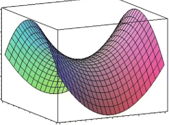
To simplify the discussion without loss of generality, we suppose that A is a 2 × 2 matrix with eigenvalues λ₁ and λ ₂. Three sign combinations of these eigenvalues are possible; both positive, both negative, or one positive and one negative. The signs of the eigenvalues determine the stability of the equilibrium point in our current problem, as illustrated in Fig. 2.2. When all eigenvalues are negative, the equilibrium point x * is stable (in Eq. (2.7), ). In stable equilibrium, x *

behaves like a jug whose potential is minimized at its base, so that all points surrounding x * are drawn toward it. In Eq. (2.7), with a single equilibrium point at , the system eventually converges to regardless of the initial conditions. If all eigenvalues are positive then

behaves like the peak of a dune (see central panel of Fig. 2.2). In this case, regardless of the initial conditions, the system never attains , and the system is unstable. If both positive and negative eigenvalues exist, converges in one direction but diverges in a linearly independent direction, as shown in the right panel of Fig. 2.2. Such an equilibrium point is called a saddle point (viewed three-dimensionally in Fig. 2.3), and is also unstable.

(23)

Fig. 2.3 Saddle

In summary, the equilibrium point is the solution of the given system state equation satisfying . The signs of the eigenvalues of the transition matrix determine whether the equilibrium point

is a source, a sink, or a saddle point . Negative and positive eigenvalues give rise to sinks and sources, respectively, while mixed eigenvalues signify a saddle point. This seemingly trivial fact is of critical importance. Once the nature of the equilibrium points of a system is determined, laborious numerical calculations to find stationary solutions are not required. Estimating the system dynamics by closely examining the eigenvalues is known as the deductive approach. To reiterate, if a deductive approach is possible, there is no requirement for numerical solutions.

Thus far, Eq. (2.7) has been considered as continuous in time. We now reinterpret (2.7) as a time-discretized system and investigate its behavior. The essence of time discretization was explained in Eqs. (2.1, 2.2, 2.3, 2.4, 2.5, and 2.6).

Initially, we adopt a forward difference scheme in time. Equation (2.7) becomes

(2.9) In physical dynamical system s, a recurrence equation such (2.9), in which a linear continuous equation is discretized in time, is sometimes called a linear mapping . The transition matrix

of Eq. (2.9) is essentially equal to Eq. (2.3). For this linear mapping to be stable (non-diverging), the absolute value of the maximum eigenvalue of the transition matrix must not exceed 1. Again, the necessary and sufficient stability criterion is as follows:

Now, let us assume stability as an original system characteristic. In other words, assume that the following is true:

(2.10) The eigenvalue of the unit matrix E is 1. We know that if the eigenvalues λ _Dof a matrix D are known, the eigenvalues of a function of D, f(D), are f(λ _D). Applying this rule under the assumptions of Eq. (2.10), the transition matrix of the linear mapping becomes

(24)

satisfied. Thus, the linear mapping of an originally stable system may be unstable. This is a surprising result. It implies that even though the original qualities were good, the calculations fail because of errors introduced in subsequent “time discretization” operations. This potential instability, generated when continuous time is mapped to a discrete system, is exactly the numerical instability. We now consider the same linear mapping under backward difference time discretization. In this case, the mapping is

(2.12) from which we obtain

(2.13) This linear mapping never diverges and will not cause the numerical fluctuations. Thus, if the original qualities are good, it appears that the integrity of the system is retained under backward difference time discretization.

2.2 Non-linear Dynamical Systems

Consider a continuous dynamical system in which the system state equation s are expressed by a non-linear function f:

(2.14) The subsequent procedure is typical of how nonlinearities are treated in all types of analyses. Non-linear functions are approximated to Non-linear functions over infinitesimal intervals by Taylor expansion. Expanding the right hand side of Eq. (2.14), we get

(2.15) From the definition of equilibrium point, (this should be evident by substituting in Eq. (2.14)), Eq. (2.15) is approximately equal to

(2.16) Equation (2.16) is approximated to a linear equation as follows:

(2.17) The first term on the right of (2.17) is first-order in x, while the second term is constant. Now we can apply the deductive approach introduced in the previous section. Clearly the transition matrix is f′(x*). We must determine the signs of the eigenvalues corresponding to the equilibrium points of this matrix.

The transition matrix is the Jacobian matrix of tangent gradients of the multi-variable vector function.

(2.18)

(25)

we seek the equilibrium points of Eq. (2.14), which are solutions to in the given system state equation . A system may contain one or several equilibrium points. In general, quadratic and quartic non-linear functions possess two and four equilibrium points, respectively. Whether each of these equilibrium points ( ) is a source, a sink, or a saddle point is determined by the sign of the eigenvalues of the transition matrix (2.18). As before, if all n eigenvalues are negative, the

equilibrium point is a stable sink, if all are positive, it is an unstable source, and if a mix of signs is found, it is an unstable saddle point. The stability characteristics of the equilibrium points apply only within the vicinity of the equilibrium points (as assumed in the Taylor expansion). Hence, when several equilibrium points exist, the behavior of the system as depends on the starting point of the dynamics, i.e., the initial values. Because the linear system in Sect. 2.1 possessed a single

equilibrium point at , this type of initial condition dependency was irrelevant, but non-linear systems can depend heavily on the initial conditions.

2.3 2-Player & 2-Stratey (2 × 2) Games

In this section, the 2-player 2-strategy game (abbreviated as two-by-two game or 2 × 2 game ) is presented as an example of a non-linear system. As the reader will come to appreciate, this

apparently esoteric two-by-two game is related to environmental problems.

As previously explained, the two-by-two game is a branch of applied mathematics that models human decision making. It is a relatively new mathematical tool based on the pioneering work of von Neumann and Morgenstern entitled “Theory of games and economic behavior” published in 1944. The applications of the two-by-two game are extremely diverse, ranging from social sciences such as economics and politics to biology, information science, and physics. If a group of particles

possessing binary strategies of cooperation or defection is imposed to develop a spatial structure, clusters of cooperation particles emerge abruptly. This seems similar to formation of crystallization or phase transitions in materials. Currently, these analogies have drawn huge interest from members of the statistical physics community.

From an unlimited population, two individuals are selected at random and made to play the game. The game uses two discrete strategies (as shown in Fig. 2.4); cooperation (C) and defection (D). The pair of players receives payoffs in each of the four combinations of C and D. A symmetrical structure between the two players is assumed. In Fig. 2.4, the payoff of player 1 (the “row” player) is

represented by the entries preceding the commas; the payoff of player 2 (the “column” player) by the entries after the commas. The payoff matrix is denoted by . A player can also be called an

(26)

Fig. 2.4 Payoff matrix of 2 × 2 game

Here, the gamble-intending dilemma (hereafter referred to as GID ) and risk-averting dilemma (hereafter referred to as RAD ) are introduced. The existence of these dilemmas is determined by D_g

and D_r, defined as follows4_:

(2.19) If D _g > 0, GID behavior results, while D _r > 0 leads to RAD . Each of the dilemma classes and the existence of GIDs and RADs are summarized in Fig. 2.5. Although, the reader may be

overwhelmed at this point having been introduced to a large set of qualities without proofs or detailed explanations, we request the reader to bear with this for just a little bit longer. GIDs are sometimes called Chicken dilemmas while RIDs can be referred to as SH dilemmas. Figure 2.5

shows that the PD game may be Chicken or SH (details will be provided later).

Fig. 2.5 Class type in 2 × 2 game

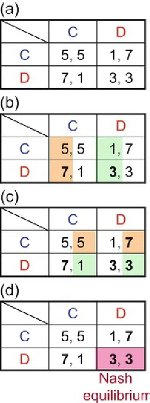
A couple of further explanations are needed here.

Figure 2.6(a) shows a game setup of the prisoner’s dilemma (PD ) class. Calculating D_g and D_r

(27)

is known as the Nash equilibrium. In this example, the Nash equilibrium indicates the grouping of rational strategies adopted by an agent selected at random from an unlimited agents who participates in a single game. Figure 2.6 reveals that both agents exhibit D behavior, and defect each another to accept low profit P (also from that figure, the relationship T > R > P > S is seen to hold in PD).

Relating this outcome to the non-linear dynamics of the previous section, even if the unlimited agents began with an even division of cooperative and defection agents (50 % cooperators & 50 %

defectors), once the game is started and the strategy of the agents reviewed according to a certain set of rules after every step5_{; as time progresses,}6_{the system will stabilize into a state in which all}

members (despite the unlimited population size) exhibit defection behavior.

Fig. 2.6 Derivation method for Nash equilibrium with PD as an example

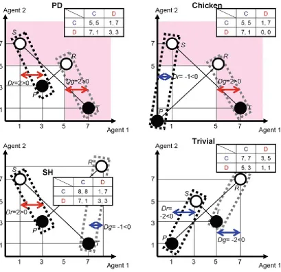
Figure 2.7 plots the payoffs for Agents 1 and 2 on the vertical and horizontal axis, respectively, and displays the payoff matrices for each of the four game classes. These diagrams show the feasible solutions regions. The pink areas within the feasible solutions of PD and Chicken reside in the 1st, 2nd, and 4th quadrant (around the central point R). When several plots exist in these regions, we hope to determine the most desirable game outcome between the equal outcomes of Agents 1 and 2. In reality, T and S are clearly the desirable outcomes for Agent 1 and his opponent, respectively.

(28)

pink region (result not shown), and a unique optimal solution exists, R.

Fig. 2.7 Feasible solution regions of each game class and examples of D_g_andD_r

In Fig. 2.7, the open and filled circles ○ and ● indicate that Agent 1 (your own offer, say), adopts C and D strategies, respectively. The C and D strategies of Agent 2 (the opponent’s offer) are

delineated by gray and black dotted lines, respectively. With this visualization, the following discussion should be apparent. In the PD game (upper left panel of Fig. 2.7), if the strategy of the opponent’s offer is fixed as C (region within the gray dotted lines), the most rational strategy for your hand is D, which lies further along the horizontal axis (indicating a higher payoff for Agent 1). If your opponent’s offer is fixed on D, the same situation arises; within the D region of Agent 2, the D

(29)

of the plots surrounded by black or gray (see upper right and lower left panels of Fig. 2.7 for Chicken and SH games, respectively).

The above dilemmas, to which we have referred so extensively, are defined in the following paragraphs.

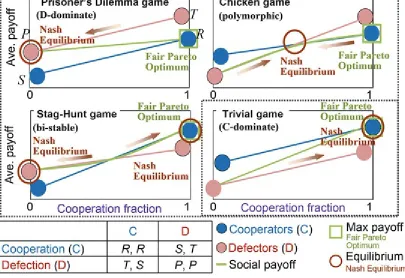
A dilemma, from mathematical meaning, is introduced whenever the Pareto optimum does not match the Nash equilibria. In PD , Chicken, and SH , the fair Pareto optimums differ from the Nash equilibria. SH yields only partial match ((C, C) is one of Nash equilibria), but causes dilemma because other outcomes are also possible. The details are explained below.

In PD , the magnitudes of the outcomes are T > R > P > S. In reverse phrasing, the order T > R > P > S characterizes the PD game class. Since D_g and D_rare both positive, GIDs and RADs coexist. The Chicken dilemma, an alternative name for the former, arises from the positive value of D_g = T − R. However, as evident from the regions of feasible solutions in the PD and Chicken games shown in Fig. 2.7, when this condition is satisfied, T and S always exist in the first, second, and fourth quadrants (assuming R as the center). Thus, it could be argued that “an incentive to exploit the opponent” exists. In a similar vein, positive D_r = P − S leads to the SH dilemma. However, when this condition is satisfied (results not schematically shown with color highlight), the feasible solution regions in Fig. 2.7 become that T and S always exist in the second, third, and fourth quadrants

(assuming P as the center), suggesting “an incentive of not being exploited by the opponent.” In fact, this situation emerged in the PD dynamics discussed earlier; as , the entire population became defection. Such an equilibrium state is called D-dominate .

In the Chicken game, T > R > S > P. Since D _g > 0 and D _r < 0, the gamble-intending (Chicken-type) dilemma exists in the absence of the risk-averting (SH -(Chicken-type) dilemma. In this game, you incur little risk of being ruined by your opponent but you may gain an advantage by exploiting the opponent. The Chicken game is characterized by S > P. That is, the most convenient situation for yourself would arise if you and your opponent adopt the D and C strategies, respectively (T > R). Conversely, if you and your opponent both adopt the D strategy, the worst outcome (P, P) results. Being ruined by your opponent would be a more favorable scenario (S > P). The structure of environmental issues is very similar. The environment is a public property available to anyone, but if overused by all individuals, it gets depleted. To preserve the environment, individuals might benefit from not using it, and hence a social dilemma is created. This supposed environment may be regarded as a public pastureland, from which your cows may be permitted to consume an unlimited or restricted amount (corresponding to defection and cooperation strategies, respectively). In the short-term, the cooperative strategy restricts the cows’ diet until the ground has recovered. This situation can be modelled as a multi-player Chicken game termed the tragedy of commons (Hardin 1968). The Nash equilibria of the Chicken game are (C, D) and (D, C), implying that if half of the population are initially cooperative,7

as , cooperation and defection members exist in certain proportions (this does not mean that specific agents are restricted to C and D strategies, but rather that the proportions of individuals adopting C and D stabilize to fixed values). This scenario is called coexistence or polymorphic equilibrium.

(30)

deer, a successful outcome is likely. However, if the opponent is not certain to cooperate (but instead might defect to cause trouble for the co-operator while knowingly losing their share of the catch), the dilemma of whether one should go on a rabbit hunt (which can be undertaken single-handedly, and is a defection strategy) arises. The name “deer hunting game” is derived from this episode in Chapter Two of “Discourse on Inequality” by Jean-Jacques Rousseau, who is famous for “The Social

Contract” and “Émile.” The deer hunting game epitomises SH. The Nash equilibria in SH are (C, C) and (D, D), but the dynamics depend on the initial proportion of cooperative individuals. As , the systems converge to either complete defection or complete cooperation. In other words, whether a dark, uncooperative society or a fully cooperative society emerges depends on the initial proportion of cooperators. This type of dynamics is known as bi-stable .

In the Trivial game, R > T > S > P, and D _gand D _rare both negative. This system is devoid of GIDs and RADs. The Nash equilibrium matches the optimal solution (C, C); thus, regardless of initial cooperation status, all members become cooperative as . This type of equilibrium is called C-dominate .

The PD game presents tough dilemmas containing both Chicken and SH -type dilemmas. Since a portion of the optimal SH solutions matches the Nash equilibria, the SH dilemma is weaker than the Chicken dilemma. As previously explained, whether a fully cooperating society emerges depends upon the initial values.

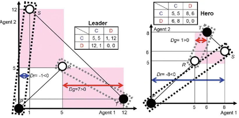
There are other several game classes. More precisely, Chicken game contains two sub-classes; one is Leader Game and another is Hero Game. Those two have polymorphic equilibriums, because D_g > 0 and D _r < 0, the gamble-intending (Chicken-type) dilemma exists in the absence of the risk-averting (SH -type) dilemma. The feasible solutions regions of those two are shown in Fig. 2.8.

Fig. 2.8 Feasible solution regions of Leader and Hero Games

Crucially important feature of those games is S + T > 2R is always satisfied. Only the difference to identify those two is the order of T and S. If T > S is valid, it is a Leader game. It is a Hero game, if S > T is valid. Those two types of 2 × 2 game s are very special. It is because, unlike PD ( D_g > 0 & D

r > 0, and S + T < 2R) and pure Chicken (Dg > 0 & D r < 0, and S + T < 2R), continuing mutual

(31)

The fair Pareto optimum in the cases is obtaining T (S) followed with S (T) in an entire alternating way ( ST-reciprocity ). In this point, we cannot evaluate a social efficiency by a cooperation rate, which is measured by cooperators fraction among the mother population, anymore. Instead, we have to take average payoff of all game players. Summing up, we should say that both Leader and Hero games have Chicken-type dilemma, and are expected to realize ST-reciprocity to attain the fair Pareto optimum unlike PD and pure Chicken favoring R-reciprocity. We will deliberately discuss about R -reciprocity and ST-Reciprocity latter.8

Another sub-game class to be noted is Donor & Recipient Game (sometimes abbreviated by D & R Game), where D _g > 0 & D_r>0 and D_g = D_rare satisfied. This means D & R game belongs to PD . This particular game has been used as one of the template models by theoretical biologist, because this game captures a social dilemma situation observed in many biological applications. Suppose you donate cost; c to help your game opponent. If your opponent is also willing to donate you by paying c, both of you and your opponent obtain benefit; b. Thus, the net payoff of both you and your opponent is

b – c. Contrariwise, if your opponent rejects to donate even you offering donation, your net payoff is – c (namely, you are exploited by your opponent) and that of your opponent is b. The asymmetric situation, where you and your opponent respectively offer D and C, gives you and your opponent; b

and – c, respectively. Let alone, this story can be rewritten by; P = 0, R = b −c, S = − c and T = b. Although 2 × 2 game s have four parterres; P, R, S and T, we can restrict the parameter area by fixing P and R. The most commonly accepted way is presuming P = 0 and R = 1. In this

parameterization, games are expressed by remaining two variables; T = 1 + D _gand S = − D_r. Thus, the games are parameterized by only D_g and D_r. Figure 2.9 shows all the game classes above

mentioned in D_g − D_rplane.

Fig. 2.9 Game classes of 2 × 2 game for varying D_g_andD_r_{in case}R = 1 and P = 0

2.4 Dynamics Analysis of the 2 × 2 Game

(32)

Sect. 2.2, is adopted.

As before, we assume unlimited group size (i.e., infinite number of agents) existing in a well-mixed state with no social viscosities. The strategies (offers) adopted by an agent are cooperation (C) or defection (D), expressed by the following state vectors:

(2.20-1) (2.20-2) The payoff matrix of the game structure is

(2.21) Moreover, the proportions of agents adopting strategy C and strategy D at a given time (referred to as the strategy ratio) are defined by s ₁and s ₂ respectively. These strategy ratios are expressed as

(2.22) From the condition of simplex we get

(2.23) The validity of Eqs. (2.20-1, 2.20-2, 2.21, 2.22, and 2.23) should be understood from the

following matrix equation describing the battle between two agents adopting strategy D, in which the outcome is P:

(2.24) A variant form of Eq. (2.24) also computes the payoff when one strategy plays a game M against another with a different strategy. The expected payoff when an agent using strategy C battles with a randomly sampled agent at the present time expressed as strategy ratio s is

Similarly, the expected payoff when an agent using strategy D fights a randomly sampled agent at the present time expressed as strategy ratio s is

The replicator dynamics are defined as the strategy ratio dynamics of strategy i, expressed as

(33)

strategy ratio) will increase in the next time step, whereas less successful strategies will decrease. The ratio of this extent is thought to be decided by comparing with the aforementioned level of “success.” In such a system, good conduct is rewarded whereas bad conduct is punished (a form of survival of the fittest). Selection mechanisms in the natural world (including human social systems) tend to operate in this manner. Alternative systems of rewarding the good and punishing the bad exist in which the response to the acquired payoffs differs from that of Eq. (2.25) may be possible. Also randomness caused by luck may enter the dynamics (i.e., poor-scoring individuals could, if lucky enough, produce offspring). In any case, we suppose replicator dynamics as the “set of rules” in the following analysis.

Substituting Eqs. (2.20-1, 2.20-2, 2.21, and 2.22) into Eq. (2.25) and explicitly writing the elements, we obtain

(2.26) Note that when the right hand side of (2.26) = 0, the equation becomes a cubic in s₁ and s₂ ; that is, the system contains three equilibrium points. Two of these are self-evident:

(2.27-1)

(2.27-2) In the former, all individuals ultimately become cooperative; the latter leads to the defection state, implying C-dominant and D-dominant, respectively. The remaining equilibrium point is obtained by simultaneously solving Eq. (2.26), setting […] on the right hand side to 0 and eliminating s ₂ through Eq. (2.23) (the reader should confirm this for themselves):

(2.27-3) This third equilibrium point lies within [0, 1] depending on the values of P, R, S, and T. In this case, the dynamics become polymorphic or bi-stable . Equation (2.27-3) defines an internal

equilibrium point.

Once the three equilibrium points are obtained, the signs of the eigenvalues of the Jacobian matrix at each equilibrium point are determined, and the equilibrium points are assessed as sink, source, or saddle.

To this end, we re-write Eq. (2.26) as follows:

(2.28-1) (2.28-2) From Eq. (2.23), we observe that . Hence, the Jacobian (2.18) is calculated as

(34)

1.

2.

3.

is a 2 × 2 matrix, so its eigenvalues (0 and ) are easily obtained

using senior school mathematics (readers should try to recall and apply the eigenvalue calculations from their maths textbooks). Since 0 is unsigned, we need only obtain the sign of to establish the equilibrium conditions. Explicitly, these eigenvalues are

(2.30)

The necessary and sufficient condition for the equilibrium point s*| _C-dominate to be sink is when substituting into Eq. (2.30). The following conditions are sought:

(2.31)

The necessary and sufficient condition for the equilibrium point s*| _D-dominate to be a sink is when substituting into Eq. (2.30). We now require that

(2.32)

The necessary and sufficient conditions for the equilibrium point s*|_Polymorphic to be a sink is

with substituted into Eq. (2.30). Noting that , we seek

the following conditions:

(2.33)

The above conditions are summarized in Table 2.1, with the following substitution:

Table 2.1 2 × 2 game dynamics derived analytically

Game class Phase Nash equilibrium Sign of D_gSign of D_rEach point sink, source, or saddle (1,0) (0,1)

PD D-Dominate (0,1) + + Source Sink Saddle

Chicken Polymorphic + − Source Source Sink

SH Bi-stable (0,1) or (1,0) − + Sink Sink Source

(35)

Defining D _gand D _rin Eq. (2.19), the four game classes were established as PD , Chicken, SH , and Trivial (see Fig. 2.5). Here, these divisions are represented by the difference between the signs of the three equilibrium points.

In PD , s*| _C-dominate and s*| _D-dominate are source and sink, respectively; hence, regardless of the initial cooperation proportion in [0, 1] the ultimate state is one of complete defection at .

In Chicken, s*| _C-dominate and s*| _D-dominate are both sources. In this case s*|_Polymorphic (value in [0, 1]) is a sink, so regardless of initial cooperation proportion, as , the system settles to the internal equilibrium point s*|_Polymorphic. As previously mentioned, this state does not imply that specific agents are fixed into cooperation or defection strategies, but that when the infinitely large group is viewed as a whole, the proportions of cooperation and defection players are (dynamically) steady.

In SH , the internal equilibrium point s*|_Polymorphic is a source, while s*| _C-dominate and s*| _D-dominate are both sinks. Therefore if the initial proportion of cooperative players is smaller (or larger) than s*|_Polymorphic, the ultimate state is pure defection, (or pure cooperation), and the system is bi-stable .

In Trivial, s*| _C-dominate is a sink and s*| _D-dominate is a source, so regardless of the initial

cooperation proportion, the pure cooperation state is inevitable. For this reason, Trivial is a game with no dilemmas.

The above discussion is summarized schematically in Fig. 2.10.

Fig. 2.10 Phase diagram of dynamics classified by D_g_andD_r_{of two-by-two game and a summary of dynamics of each game class}

(left panel). Right panel; Cooperation fraction at equilibrium when an infinite and well-mixed population with replicator dynamics is assumed when initial cooperation fraction; P_c_{of 0.5 presuming. PD and Trivial are colored with}blue and red, respectively, since D-dominate and C-D-dominate phases are established. In Chicken game region, gradually shifting of cooperation fraction at equilibrium is observed due to polymorphic phase. In SH game region, bi-stable shows twofold phases; either absorbed all cooperation bor all defection

Here, we have fully characterized the 2 × 2 replicator dynamics , expressed as non-linear cubic equations.

(36)

dynamics are relatively simple, and one of the equilibrium points inevitably acts as a sink. If the number of strategies is increased, more degrees of freedom are introduced, leading to perturbation dynamics (which display periodic behavior) or chaos (which is deterministic but unpredictable). The interested reader should take a look at related literatures (Weibull 1997; Nowak 2006a).

2.5 Multi-player Games

Though we have so far assumed that there are two game players, a multi-player situation is more typical in a realistic context. It is therefore natural that the discussion can now be extended to multi-player games.

First, we outline the so-called Public Goods Game (PGG ), which has been used most often in the field as a template for multi-player games. This game is based on a social dilemma around a public good that can only be sustained by a reasonable number of moral-minded cooperators through their donations. This means players have an incentive not to donate but also to want to get their share of the cooperative fruits brought about by the donations of others.

Suppose G players participate in a single multi-player game, where a cooperator is requested to donate a cost c (in most cases, as in Fig. 2.11, assuming c = 1) to a public pool. The number of cooperators is denoted by n_c . After collecting the donations from all cooperators among the G

players, the total pooled donation is multiplied by an amplifying factor, r. Thus, the public good is amplified. The fruits of this public good are distributed equally to all game participants irrespective of whether they are a cooperator or defector. In this sense, a defector can be called a free-rider .9

Here, we can define the payoff structure functions for both cooperators and defectors as shown in Fig. 2.11, which can be drawn from the cooperation fractions in the lower panel of Fig. 2.11. One important thing is that the defectors’ payoff is always larger than that of the cooperators at any particular cooperation fraction. This schematic relation is redrawn more precisely in Fig. 2.12, where the cooperator and defector plots indicate the respective payoffs at discrete cooperation fractions, where P_c = n _c/G. The figure obviously suggests that, as long as is satisfied, a cooperator has no incentive to keep cooperating at any cooperation fraction, and thus the cooperation fraction is always declining regardless of the initial cooperation fraction. Consequently, Nash equilibrium is absorbed by an all defectors state, i.e., P_c = 0. On the other hand, the maximum social payoff, or fair Pareto optimum, appears at the all cooperators state, P_c = 1. This is why we can basically identify PGG as multi-player Prisoner’s Dilemma ( N-PD ) game. Comparing with 2 × 2

(37)

Fig. 2.11 Public Goods Game (PGG ); N-Prisoner’s Dilemma Game

Fig. 2.12 Payoff structure function of multi-player PD

(38)

Fig. 2.13 Four game classes and payoff structure functions of multi-players games

Multi-player Chicken (N-Chicken) is featured when the cooperator’s payoff function crosses with the defector’s one at a certain cooperation fraction, which is called an internal equilibrium point, as in 2 × 2 Chicken. As mentioned before, a multi-player Chicken game termed “the tragedy of commons ” has been accepted as one of the typical template models for describing a social dilemma caused by environmental problems.10_{Multi-players Stag Hunt (}_N_{-SH ) games also have a crossing point}

between the two payoff functions. But the dynamics differ from those of N-Chicken, as shown schematically in the figure. Multi-player Trivial (N-Trivial) has no social dilemma, since

cooperation dominates defection meaning the cooperator’s payoff exceeds the defector’s one at any cooperation fraction.

2.6 Social Viscosity; Reciprocity Mechanisms

As long as an infinite and well-mixed population is assumed, the theory correctly predicts the

dynamics of any symmetric 2-strategy game as well as its equilibrium as we discussed in Sects. 2.5

and 2.6.

Although the fundamental theory seems transparent and unsurprising, the interdisciplinary field around the study of evolutionary games has been persistent, with a new paper appearing every day, or even every hour or minute. What has aroused this enthusiasm to study the field in mathematicians, biologists, physicists, information scientists, and even common foot soldiers such as the author? At the end of the day, it comes down to a single question: What additional mechanisms will promote the ultimate cooperation among agents if a pair of agents is randomly selected from an unlimited group (i.e., an infinite and well-mixed selection) and forced into a specified game (such as PD )? In the natural world, cooperative behavior is found not only in human societies, but also among social

(39)

From recent theoretical studies, the puzzle of what can be “supplementary framework” of dilemma resolution has been unfolded. Nowak (2006b) showed there are the five fundamental protocols to mitigate or cancel dilemmas,11_{summarized as in Fig.}_2.14_{. The mechanisms of these}

activities are governed by very ordinary and beautiful mathematical expressions similar to those of kin selection (Hamilton 1963). Nowak refers to these mechanisms as “Social Viscosity.” Under these circumstances, the population is initially well-mixed as before, and each game is played by a single person whose next encounter is unknown. But, in repeated game battles between a pair of individuals (direct reciprocity ),12_{or observing the tag of the opponent (indirect reciprocity ), the behaviour of}

opponent; cooperation or defection, can be distinguished. Or, when players play games against only the neighboring players throughout the network, information relating to strategy is obtained (network reciprocity ). All these enable the agents to overcome the dilemmas and create a cooperative

society.13_{These processes essentially reduce the anonymity from that of an infinite and well-mixed}

population (which exists in a total anonymous state) and authenticate the battle opponent. By carefully studying the authentication of others through indirect reciprocity, it may be possible to elucidate how notable features of organisms (such as colour differences in bird crests) evolve, or evolution of language, which is the ultimate third party identification system. Network reciprocity may also help us understand the structure of special network topologies such as the scale-free graphs observed in many natural phenomena, as well as human social systems; in particular, how cooperation self-organizes in such networks.

Fig. 2.14 Five basic mechanisms of dilemma resolution and example of Network Reciprocity

2.7 Universal Scaling for Dilemma Strength in 2 × 2 Games

As long as an infinite and well-mixed population is presumed with the replicator dynamics , an

evolutionary trail can be stipulated strictly by what Table 2.1 shows. In a nutshell, whenever both D_g

and D_rare fixed, the evolutionary dynamics are determined. In this sense, D_gand D_rare scaling parameters of dilemma strength, and the dynamics of equilibrium are determined by their values.

(40)

details of simulation setting are described later). Although these three games have the same D _gand D

r, cooperation fractions in Fig. 2.15 are completely different depending on the value of R − P. The

larger R − P becomes, the higher is the equilibrium cooperation fraction.

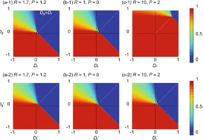
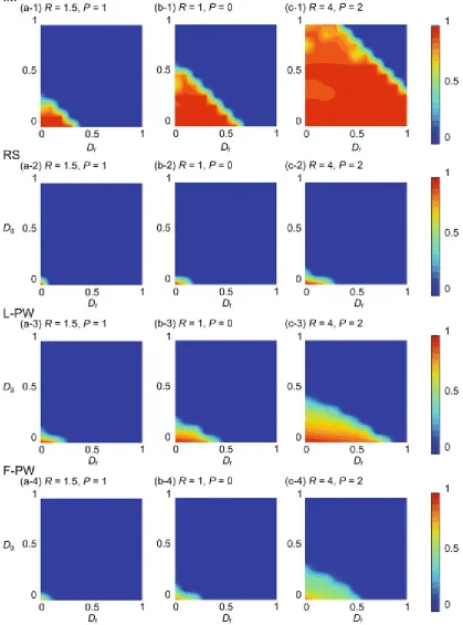
Fig. 2.15 Averaged cooperation fraction D_r₋D_g_{diagrams for (}a) R = 1.5, P = 1, (b) R = 1, P = 0, and (c) R = 4, P = 2. Games are played on 8-neighbor lattice . Imitation Max (IM) is adopted as the strategy update rule

Thus, in a game with a certain reciprocity mechanism, the dilemma strength cannot be quantified only by D _gand D _r, which can be sufficient indicators in an infinite well-mixed population game. Let us assume two PDs having the same D _gand D _r, as shown in Fig. 2.16, which visually explains the preceding discussion. As R − P becomes larger relative to D _gand D_r, we can regard and

asymptotically. This is similar to the Avatamasaka game, defined by Akiyama and Aruka (2004), wherein a focal player’s gain becomes irrelevant to his own offer, but is entirely dominated by his opponent’s offer. Thus, in game (b), the payoff increment of the focal player by his offering either cooperation (C) or defection (D) is relatively lower than that of whether his opponent offering cooperation (C) or defection (D). This is because the focal player’s payoff is affected more by his opponent’s offer than by his own decision, whether C or D. Thus, we can say that game (b) has a relatively higher incentive to establish a reciprocal relationship than does game (a). Therefore, we should take R − P into a new index parameter to evaluate dilemma strength when a game is played in a situation with social viscosity , wherein an agent might play with the same opponent in several rounds; because of a reciprocity mechanism.