Department of Statistics STA1501 Descrip (1)

(1)

Department of Statistics

STA1501

Descriptive Statistics and Probability

(2)

(3)

(4)

CONTENTS

ORIENTATION vi

STUDY UNIT 1

1.1 Introduction 1

What is Statistics?

1.2 Types of Data and Information 4

1.3 Self-correcting Exercises for Unit 1 8

1.4 Solutions to Self-correcting Exercises for Unit 1 10

1.5 Learning Outcomes 12

1.6 Study Unit 1: Summary 13

STUDY UNIT 2

2.1 Introduction 14

2.2 Graphical and Tabular Techniques to describe Nominal Data 14

2.3 Graphical Techniques to Describe Interval data 18

2.4 Describing the Relationship between Two Variables and Describing Time Series Data 24

STUDY UNIT 3

3.1 Introduction 34

3.2 Graphical Excellence and Graphical Deception 34

3.3 Presenting Statistics: Written Reports and Oral Representations 40

3.4 Measures of Central Location 40

3.5 Measures of Variablity 45

STUDY UNIT 4

4.1 Introduction 58

4.2 Measures of Relative Standing and Box Plots 59

4.3 Measures of Linear Relationship 62

4.4 Comparing Graphical and Numerical Techniques 64

4.5 General Guidelines for Exploring Data 64

(5)

STUDY UNIT 5

5.1 Introduction 70

5.2 Methods of Collecting Data and Sampling 70

5.3 Sampling Plans 72

5.4 Sampling and Nonsampling Errors 81

STUDY UNIT 6

6.1 Introduction 91

6.2 A basis for probability 92

6.3 Sophisticated methods and rules in probability theory 96

6.4 The rule of Bayes 108

STUDY UNIT 7

7.1 Introduction 116

7.2 Discrete probability distributions 117

7.3 Bivariate distributions 122

7.4 Binomial distribution 127

7.5 Poisson distribution 131

STUDY UNIT 8

8.2 Continuous probability distributions 138

8.3 Continuous probability distributions: Normal distribution 140

8.4 Other Continuous probability distributions 155

(6)

STUDY UNIT 9

9.2 Sampling distribution of the mean 166

9.3 Sampling distribution of a proportion 172

9.4 Sampling distribution of the difference between two means 179

9.5 Self-Correcting Exercises for Unit 9 183

9.6 Solutions to Self-Correcting Exercises for Unit 9 184

STUDY UNIT 10

10.2 Concepts of Estimation 190

10.3 Estimating the Population Mean when the Population Standard Deviation is Known 192

10.4 Selecting the Sample Size 198

STUDY UNIT 11

11.2 Concepts of Hypothesis Testing 210

11.3 Testing the Population Mean when the Population Standard Deviation is Known 213 11.4 Calculating the Probability of a Type II error 221

11.5 The Road Ahead 224

11.6 Self-Correcting Exercises for Unit 11 224

11.7 Solutions to Self-Correcting Exercises for Unit 11 225

STUDY UNIT 12

12.2 Inference about a Population Mean when the standard deviation is unknown 229 12.3 Inference about the mean: What else need you keep in mind? 242

12.4 Inference about a Population Variance 244

12.5 Inference about a Population Proportion 247

(7)

ORIENTATION

Introduction

Welcome to STA1501. This module consits of the ﬁrst half of the ﬁrst-year statistics course for students in the College of Economic and Management Sciences. The two modules form an integrated whole and are focused on the following objective: To collect, organise, analyse and interpret data for the purpose of making better decisions.

STA1501 STA1502 STA1503

This is where you are

First−year Statistics

The first part of the module covers the “Descriptive Statistics” part, which is earthly and real and the focus is on the presentation of data. Thefirst step is to carefully think about thetype of variable that each measurement represents. This is extremely important as the type dictates what you can or can’t do in the rest of your data analysis. Then we will also consider thecollectionof data (which most often, for the social sciences and in business applications, involve administering questionnaires and/or survey data, and sampling plays an important role in this regard). Between thecollection of data and the ultimate goal of analysis of data lies the very important step of organising and summarising the data. So, in this module we discuss how weorganise and summarise the gathered information intelligibly and efficiently.

The second part of the module covers the“Probability and Probability Distributions” part where we leave the practical familiarity of data and turn to the less familiar abstract concept of probability. This is almost like a shift in gears! A proper understanding of the laws of probability is essential to ensure a proper understanding of the mechanisms underlying statistical data analysis. Probability theory is the tool that makes statistical inference possible.

(8)

a successp. These critical values are calledparameters. We most often don’t know what the values of the parameters are and thus we cannot “utilise” these distributions (i.e. use the mathematical formula to draw a probability density graph or compute speciﬁc probabilities) unless we somehow

estimate these unknown parameters. It makes perfect logical sense that to estimate the value of an unknown population parameter, we compute a corresponding or comparable characteristic of the sample.

(9)

Learning objectives

There are very specific outcomes for this module which we list below. Throughout your study of this module you must come back to this page, sit back and reflect upon these outcomes, think them through, digest them into your system and feel confident in the end that you have mastered them.

• Analyse data considering different types of data and how they relate to relevant graphical and tabular presentations e.g. pie charts, bar charts, histograms, stem-and-leaf displays, line charts, scatter diagrams and box-and-whisker plots

• Analyse data by calculating accurate numerical measures of central location, variability, relative standing and linear relationship.

• Differentiate between simple random sampling, stratiﬁed random sampling and cluster sampling and implement a sampling plan for a given research problem with an awareness for the effect of sampling errors.

• Describe the different concepts and laws of probability and apply deﬁnitions of joint, marginal and conditional probability.

• Apply the complement, multiplication and addition rules and probability trees for calculation of more complex events and calculate complicated events from the probabilities of related events.

• Understand the role of probability in decision making and the application in basic statistical inference.

• Describe random variables and the probabilities associated with them in the form of a table, formula or graph and also in terms of its parameters, usually the expected value and the variance.

• Describe different probability distributions as either discrete or continuous and know the parameters of expected value and variance

The prescribed textbook

For this module you must studytwelve chaptersfrom theprescribed textbook:

Keller,G.(2009, (8thedition))

Managerial Statistics,South–Western, Cengage Learning Chapter 1: WHAT IS STATISTICS?

Chapter 2: GRAPHICAL AND TABULAR DESCRIPTIVE TECHNIQUES Chapter 3: ART AND SCIENCE OF GRAPHICAL PRESENTATIONS Chapter 4: NUMERICAL DESCRIPTIVE TECHNIQUES

Chapter 5: DATA COLLECTION AND SAMPLING Chapter 6: PROBABILITY

(10)

Chapter 8: CONTINUOUS PROBABILITY DISTRIBUTION Chapter 9: SAMPLING DISTRIBUTIONS

Chapter 10: INTRODUCTION TO ESTIMATION

Chapter 11: INTRODUCTION TO HYPOTHESIS TESTING Chapter 12: INFERENCE ABOUT A POPULATION

The study guide

The study guide is exactly what its name implies: a guide through the textbook in a systematic way. The textbook will focus on the theoretical contents of the module and we have tried not to duplicate material from the textbook in the guide. For each separate study unit you shouldﬁrst study the work in the textbook and utilise the guide to assess your progress, test your knowledge and prepare for the examination. In other words, the study guide will provide you with an opportunity to apply your knowledge of the material that is covered in the textbook.

This study guide serves as an interactive workbook, where spaces are provided for your convenience. Should you so prefer, you are welcome to write and reference your solutions in your own book orﬁle, if the space we supply is insufﬁcient or not to your liking.

Study units and workload

We realise that you might feel overwhelmed by the volumes and volumes of printed matter that you have to absorb as a student! How do you eat an elephant? Bite by bite! We have divided the twelve chapters of the textbook into 12 study units or “sessions”. Make very sure about the sections in each study unit since some sections of the textbook are not included and we do not want you frustrated by working through unnecessary work. The study units vary in length but you should try to spendon average 12 hours on each unit. Practically everybody should be able to do statistics. It depends on the amount of TIME you spend on the subject. Regular contact with statistics will ensure that your study becomes personally rewarding.

Try to work through as many of the exercises as possible

Doing exercises on your own will not only enhance your understanding of the work, but it will give you confidence as well. Feedback is given immediately after the activity to help you check whether you understand the specific concept. The activities are designed (i.e. specific exercises are selected) so that you can reflect on a concept discussed in the textbook. You can only obtain maximum benefit from this activity-feedback process if you discipline yourselfnot to peep at the solution before you have attempted it on your own!

Final word: Attitude

(11)

effort. However, we do claim that knowledge of statistics will enable you to make effective decisions in your business and to conduct quantitative research into the many larger and detailed data sources that are available. Statistical literacy will enable you to understand statistical reports you might encounter as a manager in your business. We are there to assist you in a process where you shift yourself from a supported school learner to an independent learner. There will be times when you feel frustrated and discouraged and then only your attitude will pull you through!

In a paper by Sue Gordon1 (1995) from the University of Sydney, the following metaphor is given: “The learning of statistics is like building a road. It’s a wonderful road, it will take you to places you did not think you could reach. But when you have constructed one bit of road you cannot sit back and think ‘Oh, that’s a great piece of road!’ and stop at that. Each bit leads you on, shows the direction to go, opens the opportunity for more road to be built. And furthermore, the part of the road that you built a few weeks ago, that you thought you wereﬁnished with, is going to develop potholes the instant you turn your back on it. This is not to be construed as failure on your part, this is not inadequacy. This is just part of road building. This is what learning statistics is about: go back and repair, go on and build, go back and repair.”

A few logistical problems

Decimal comma or point?

We realise that in the South African schooling system commas are used to indicate the decimal digit values. You have been penalised at school for using a point. Now we sit between two ﬁres: the school system and common practice in calculators and computers! Most computer packages use the decimal point (ignoring the option to change it) and Keller (the author) also uses the decimal point in our textbook (Managerial Statistics). Thus, we shall use the decimal point in our study guide, assignments and the examination.

Role of computers and statistical calculators

The emphasis in the textbook is well beyond the arithmetic of calculating statistics and the focus is on the identiﬁcation of the correct technique, interpretation and decision making. This is achieved with aﬂexible design giving both manual calculations and computer steps.

Every statistical technique that needscomputationis illustrated in a three-step approach: Step 1 MANUALLY

Step 2 EXCEL Step 3 MINITAB

(12)

using a computer is that you can do calculations for larger and more realistic data sets. Whether you use a computer program or a statistical calculator as tool for your calculations is irrelevant to us. However, the emphasis in this module will always be on the interpretation and how to articulate the results in report writing.

(13)

Key Terms/Symbols

Sampling distribution Central limit theorem

Sampling distribution of the sample mean Standard error of the mean

Normal approximation of the binomial distribution Continuity correction factor

Sampling distribution of the sample proportion Standard error of the proportion

(14)

STUDY UNIT 1

1.1 Introduction

The objective of Statistics is to draw conclusions about a population based on the limited information contained in a sample. In other word statistics is a method to convert data into information.

READ THROUGH

Keller Chapter 1 What is Statistics? Introduction

1.1 Key Statistical concepts

1.2 Statistical Applications in Business 1.3 Statistics and the Computer

You need not panic when all the new terms do not make sense to you, neither need you remember them all at this stage! As we proceed chapter by chapter and you start applying the different techniques you will understand more. In study unit 5 you will learn most you need to know about data collection and sampling to obtain optimum information and you will learn that there are good and bad ways of obtaining a sample.

Activity 1.1

State whether the following statements are correct or incorrect.

(a) When the purpose of the statistical inference is to draw a conclusion about a population, the signiﬁcance level, as a measure of reliability, measures how frequently the conclusion will be correct in the long run.. . . . . . . .

(15)

(c) The conﬁdence level is the proportion of times that an estimating procedure will be wrong.. . . . . . . .

(d) Conclusions and estimates about a population based on sample data are not always going to be correct. For this reason measures of reliability, such as the signiﬁcance level and the conﬁdence level, should be built into the statistical inference.. . . . . . . .

(e) A university employs 2500 faculty and staff. To ascertain how the employees feel regarding a health insurance plan, 250 of the employees are surveyed. The proportion of the 250 employees who favour the health insurance plan is a parameter.. . . .

. . . .

(f) In a sample of 400 students in a college of business, 120 of them or 30% are marketing majors. The 30% is an example of statistical inference as opposed to descriptive statistics.. . . .

. . . .

(g) A population is the totality of items or things of interest under consideration.. . . . . . . .

(h) Twenty-ﬁve percent of a sample of 200 tennis players indicated that their parents did not play tennis. Based on this sample, we estimate that the 25% ﬁgure holds for the parents of all professional tennis players. This is an example of descriptive statistics as opposed to statistical inference.. . . . . . . .

(16)

Feedback

(a) Incorrect (b) Correct (c) Incorrect (d) Correct (e) Incorrect

(f) Incorrect (g) Correct (h) Incorrect

(i) Correct

READ THROUGH

Keller Chapter 1 What is Statistics?

Appendix 1.A Instructions for the CD-ROM Appendix 1.A Instruction to Microsoft Excel

At this stage we only want you to be aware of Microsoft Excel and of the fact that the CD contains an additionalstatistical software add-infor Excel which wiil enable you to do all the statistical procedures that is covered in the textbook. You can always come back to these pages when you need to know something more about Excel.

(17)

1.2 Types of Data and Information

STUDY

Keller Chapter 2 Graphical and Tabular Descriptive Techniques 2.1 Types of Data and Information

Always remember that the type of data dictates what you can or can’t do in the rest of your data analysis. (Page to the inside cover of your textbook and notice that even the cryptic complete overall summary is organised according to data types.)

Knowing about variable types and collecting data is almost like a chicken-and-egg situation! Which one comes ﬁrst? It is extremely important to carefully think about the type of variable that each measurement represents, because it could inﬂuence the manner in which the measurements will be obtained. For example, suppose you compile a questionnaire where the respondent can tick one of the following age categories:

Age Please Tick 20–25

25–35 35–45 45–65

The resulting data will be considered asordinal measurements(i.e. if ages are artiﬁcially grouped into categories).

(18)

Activity 1.2

For each of the following examples of data, determine the type:

(a) marital status. . . . . . . .

(b) rating of our study material: excellent, good, fair or poor . . . . . . . .

(c) the red blood cell count of a person. . . . . . . .

(d) the mass of an automobile. . . . . . . .

(e) the number of people per family unit. . . . . . . .

(f) the number of TV sets sold by each branch of a chain store. . . . . . . .

(g) personality type: introvert vs. extrovert. . . . . . . .

Feedback

(19)

Activity 1.3

Markinor asked 2000 adult South Africans the following question: “Do you think that you are now

ﬁnancially better off than a year ago?” The responses were

Better off 30%

The same 20%

Worse off 50%

(a) Is this an example of a nominal level of measurement? Why (not)?

. . . . . . . . . . . .

(b) Are the categories mutually exclusive? Why (not)?

. . . . . . . . . . . .

(c) Are the categories exhaustive? Why (not)?

(20)

Feedback

(a) No. With nominal data, the observations are sorted into categories with no particular order to the categories. Since we may presume that “Better off” is ranked higher than “The same” and that “The same” is ranked higher than “Worse off” I would say that this is an example of ordinal measurements.

(b) Yes. In general, categories are called mutually exclusive if each individual or object appears in only one category. It is clear that each individual can fall in only one of the three categories. You cannot be “better off” and “worse off” at the same time.

(c) Yes. In general, categories are exhaustive if the categories cover all possible outcomes. In other words each individual must appear in at least one of the categories – almost like asking “Well, what else could yourﬁnancial state be?” So, I would say yes.

Activity 1.4

At the end of an escorted travel bus vacation to Cape Town, the tour operator asks the vacationers to respond to the questions listed below. For each question, determine whether the possible responses are interval, nominal, or ordinal.

(a) How many escorted vacations have you taken prior to this one?. . . . . . . .

(b) Do you feel that your stay in Cape Town was sufﬁciently long?. . . . . . . .

(21)

(d) What is the maximum number of hours per day that you would like to spend travelling by bus?. . . . . . . . .

(e) Would your overall rating of this tour be excellent, good, fair or poor?. . . . . . . .

Feedback

(a) Interval (b) Nominal (c) Nominal (d) Interval (e) Ordinal

1.3 Self-correcting Exercises for Unit 1

Question 1

Deﬁne each of the following statistical terms: (a) Descriptive statistics

(b) Statistical inference (c) Conﬁdence level (d) Signiﬁcance level (e) Population

(22)

Question 2

A manufacturer of children toys claims that less than 3% of his products are defective. When 500 toys were drawn from a large production run, 5% were found to be defective.

(a) Deﬁne the

(i) population of interest (ii) sample

(iii) parameter (iv) statistic

(b) Does the value 3% refer to the parameter or the statistic? Why? (c) Does the value 5% refer to the parameter or the statistic? Why?

(d) Explain brieﬂy how the statistic can be used to make inferences about the parameter to test the claim.

Question 3

(a) The Human Resources Director of a large insurance company wishes to develop an employee health beneﬁts package and decides to select 400 employees from a list of all employees in order to study their preferences for the various components of a potential package. The 400 employees who will participate in this study constitute the __________.

(b) The Human Resources Director of a large hospital in Gauteng wishes to develop an employee health beneﬁts package and decides to select 300 employees from a list of all employees in order to study their preferences for the various components of a potential package. Information obtained from the sample will be used to draw conclusions about the true population __________.

Question 4

A businessman who is running for the vacant City Mayor seat with 25 000 registered voters conducts a survey. In the survey, 55% of the 500 registered voters interviewed say they planned to vote for him.

(a) What is the population of interest? (b) What is the sample?

(23)

Question 5

(a) Provide one example of nominal data. (b) Provide one example of ordinal data. (c) Provide one example of interval data

1.4 Solutions to Self-correcting Exercises for Unit1

Question 1

(a) Descriptive statistics deals with methods of organizing, summarizing, and presenting data in a convenient and informative way.

(b) Statistical inference is the process of estimation, prediction or decision making about a population, based on sample data.

(c) The conﬁdence level is a measure of reliability that measures the proportion of times that an estimating procedurewill be correct.

(d) The signiﬁcance level is a measure of reliability that measures how frequently the conclusion about a populationwill be wrong in the long run.

(e) A population is the group of all items of interest to a statistics practitioner. Populations are frequently very large and may, in fact, be inﬁnitely large.

(f) A sample is a set of data drawn from the population.

Question 2

(a) (i) The complete production run of toys.

(ii) The 500 toys drawn from the production run.

(iii) The proportion of the production run toys that are defective. (iv) The proportion of sampled toys that are defective.

(24)

Question 3

(a) sample (b) parameters

Question 4

(a) The political choices of the 25 000 registered voters.

(b) The political choices of the 500 registered voters interviewed.

(c) It is a statistic, since it is a summary measure that is computed from the sample.

Question 5

(a) Nominal data example: Political party afﬁliation for American voters recorded using the code: 1 = Democrat, 2 = Republican and 3 = Independent.

(b) Ordinal data example: Response to market research survey measured on the Likert scale using the code: 1 = Strongly agree, 2 = Agree, 3 = Neutral,

4 = Disagree and 5 = Strongly disagree.

(c) Interval data example: Temperature on the rugbyﬁeld during the Super Twelve competition.

Key terms

(25)

1.5 Learning Outcomes

Use the following learning outcomes as a checklist after you have completed this study unit to evaluate the knowledge you have acquired.

Can you

• deﬁne the following terms? - population

- sample

- parameter

- statistic

- statistical inference

• describe the different types of variables? - nominal

- ordinal

(26)

1.6 Study Unit 1: Summary

I. Statistics is the science of collecting, organizing, presenting, analyzing, and interpreting data to assist in making more effective decisions.

II. There are two types of statistics:

A. Descriptive statisticsare procedures used to organize and summarize data.

B. Inferential statisticsinvolve taking a sample from a population and making estimates about a population based on the sample results.

1. A population is an entire set of individuals or objects of interest or the measurements obtained from all individuals or objects of interest.

2. Asampleis part of the population. III. There are two types of variables:

A. Aqualitatitve variableis categorical or nonnumeric.

1. Usually we are interested in the number or percentage of observations in each category. 2. Qualitative data are usually summarized in graphs and bar charts.

B. There are two types ofquantitative variablesand they are usually reported numerically. 1. Discrete variables can assume only certain values, and there are usually gaps between

values.

2. Aninterval variable can assume any value within a speciﬁed range. IV. There are two levels of measurement:

A. With the nominal level, the data are sorted into categories with no particular order to the categories.

B. The ordinal level of measurement presumes that one classiﬁcation is ranked higher than another.

References

Keller, Gerald et al. (2005)Instructor’s Suite CD for the Student Edition of Statistics for Management and Economics, Belmont, CA USA: Duxbury, Thomson.

(27)

STUDY UNIT 2

2.1 Introduction

We emphasised in study unit 1 how extremely important it was to carefully think about thetype of variablethat each measurement of a data set represents because the type dictates what you can or can’t do in the rest of your data analysis. Consciously remind yourself to think about the data type whenever you are busy doing something with data.

Theﬁnal mind mapwe are working towards (after completion of Statistics 1) and which you have to make part of yourself, is given on the inside cover of your textbook.

2.2 Graphical and Tabular Techniques to Describe Nominal

Data

STUDY

Keller Chapter 2 Graphical and Tabular Descriptive Techniques

2.2 Graphical and Tabular Techniques to Describe Nominal Data

You will notﬁnd one chart in the study guide (or textbook) that looks “manually drawn” simply because all printed matter needs to be in electronic format for the production process. In pre-computer days statisticians produced the same pie and bar charts manually and you should not feel discouraged if you do not have the software to produce them, as long as you understand how to construct them. For a “manually drawn” pie chart the steps are as follows:

(i) Convert afrequency table _−→ proportional frequency table _−→ proportion₁₀₀ ×360. (ii) Find a pencil, a compass and a protractor.

(iii) Draw a circle (remember to mark the centre!) and mark the sections according to the calculations in (i).

(28)

Activity 2.1

Voters participating in an election exit poll in Minnesota (USA) were asked to state their political party afﬁliation. Coding the data as 1 for Republican, 2 for Democrat, and 3 for Independent, the data collected were as follows:

3 1 2 3 1 3 3 2 1 3 3 2 1 1 3 2 3 1 3 2 3 2 1 1 3

Construct a frequency bar chart.

Feedback

Manually

We need afrequency tablebefore we can draw afrequency bar chart.

Republican(1) Democrat(2) Independent(3) Tally marks

Frequency 8 6 11

Using Excel

0 2 4 6 8 10 12

Republican Democrat Independent

F

re

q

u

e

n

(29)

Activity 2.2

Car buyers were asked to indicate the car dealer they believed offered the best overall service. The four choices were Carriage Motors (C), Marco Toyota (M), Triangle Auto (T) and University Chevrolet (U). The following data were obtained:

T C C C C M T C U U M C M T C M M C M U T C C T U M M C C T T U C U T M M C U T

Construct a pie chart. Which car dealer offered the best overall service?

Feedback

C 3 5 .0 %

M 2 5 .0 % T

2 2 .5 % U 1 7 .5 %

It seems that Carriage Motors offered the best overall service.

Activity 2.3

(30)

Major of Graduate Number of graduates Accounting 58 Finance 42 Management 38 Marketing 52 Other 10

(a) Draw a pie chart of the number of graduates. (b) Draw a frequency bar chart.

(c) Which graph do you favour and why?

Feedback

(a) Pie chart

Accounting 29.0% Finance 21.0% Management 19.0% Marketing 26.0% Other 5.0%

(b) Frequency bar chart

0 10 20 30 40 50 60 70 Acc ou ntin g Fin an ce Ma na ge me nt Ma rke tin g Oth er Major F re q u e n cy

(31)

Activity 2.4

Complete the following sentences:

1. Bar and pie charts are graphical techniques for data. Bar charts focus the attention on the of the occurrences of the categories and pie charts emphasise the of occurrences of each category.

2. If we wish to emphasise the relative frequencies for nominal data, we draw a . 3. One of the advantages of a pie chart is that it clearly shows that the total of all the categories of

the pie adds to .

Feedback

1. Bar and pie charts are graphical techniques for nominal data. Bar charts focus the attention on the frequency of the occurrences of the categories, and pie charts emphasise the proportion of occurrences of each category.

2. If we wish to emphasise the relative frequencies for nominal data, we draw a pie chart.

3. One of the advantages of a pie chart is that it clearly shows that the total of all the categories of the pie adds to 100%.

2.3 Graphical Techniques To Describe Interval Data

STUDY

Keller Chapter 2 Graphical and Tabular Descriptive Techniques 2.3 Graphical Techniques to Describe Interval Data

For a “manually drawn” histogram you need:

(32)

Frequency distribution

The ﬁrst problem is to decide on the number of class intervals. There is an inverse relationship between the number of classes and the average frequency per interval. This means that a large number of classes could cause the frequencies of most classes to be small and that a small number of classes could cause the frequencies of most classes to be large. Too many intervals would not really summarise the data, whilst too few intervals would cause us to lose information. This is why Sturges’ formulacomes in handy to determine the number of classes.

The number of classes=1 + 3.3log(n). (Table 2.6 of the textbook gives a rough summary of this rule.)

The second step is to compute the size of the intervals or the interval width ( some textbooks talk aboutinterval length). Since the total number of intervals must include all the data from the smallest observation to the largest observation it seems logical that the class width can be calculated using

(largest value – smallest value)

number of intervals .Please note that this answer is seldom an integer, but then we compromise

and manipulate the result by rounding to an integer. The aim is toﬁnd an interval width that would also result in a convenient midpoint, especially if the histogram is drawn manually.

Theﬁnal step is to write down the classes. Keep in mind that we work with aninterval type variable and we wouldn’t like to have gaps between the classes but on the other hand we also won’t like the classes to be ambiguous. This means there should be no doubt where an observation belongs. The classes should be mutually exclusive and no observation can be classiﬁed into two different intervals. Make sure that the smallest as well as the largest observation each falls into a class.

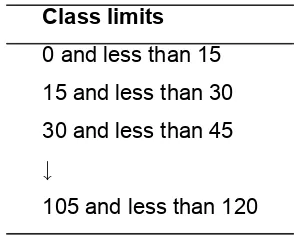
Table 2.5 in Keller actuallymeans

Class limits 0 and less than 15 15 and less than 30 30 and less than 45

↓

105 and less than 120

Compiling a frequency distribution table by hand (i.e. not using a computer) is rather cumbersome for a large sample, and one can easily make a mistake inﬁnding the smallest and the largest values. Plotting a rough stem-and-leaf display helps with the tallying and to check the calculations.

(33)

In table 2.5 of Keller (frequency distribution of long distance bills), he conveniently described the intervals as “0 to15”, “15 to30”, etc. – but strictly speaking we cannot mark the class limits as 0 – 15, 15 – 30, 30 – 45, etc. because it could be ambiguous to interpret. (These values assume possible original values and we would not be sure where a long distance bill of exactly 15 was classiﬁed.) More advanced statistical packages avoid the confusion by picking the class midpoints halfway between the two class limits and use these values on thehorizontal axis.

Activity 2.5

Complete the following sentences:

1. A frequency distribution counts the number of observations that fall into each of a series of intervals, called that cover the complete .

2. Although the frequency distribution provides information about how the numbers in the data set are distributed, the information is more easily understood and imparted by drawing a

.

3. The number of class intervals we select in a frequency distribution depends on the number of .

4. Select the correct option: Therelative frequency of a classis computed by (a) dividing the frequency of the class by the class width

(b) dividing the frequency of the class by the total number of observations in the data set (c) dividing the frequency of the class by the number of classes

5. A modal class is the class that includes the .

6. When ogives or histograms are constructed, the axis must show the true zero or origin. 7. According to Sturges’ rule, an indication of the number of class intervals in a frequency distribution

equals .

8. A bimodal histogram is one with , not necessarily equal in height.

(34)

10. A histogram is said to be positively skewed when it has a .

11. The stem-and-leaf display reveals (far more, far less) information relative to individual values than does the histogram.

Feedback

1. A frequency distribution counts the number of observations that fall into each of a series of intervals, called classes that cover the complete range of observations.

2. Although the frequency distribution provides information about how the numbers in the data set are distributed, the information is more easily understood and imparted by drawing a histogram . 3. The number of class intervals we select in a frequency distribution depends on the number of

observations in the data set.

4. Therelative frequency of a classis computed by dividing the frequency of the class by the total number of observations in the data set.

5. A modal class is the class that includes the largest number of observations.

6. When ogives or histograms are constructed, the vertical axis must show the true zero or origin. 7. According to Sturges’ rule, an indication of the number of class intervals in a frequency distribution

equals 1 + 3.3 log (n), wherenis the size of the data set.

8. A bimodal histogram is one with two peaks, not necessarily equal in height.

9. A histogram is said to be symmetric if, when we draw a vertical line down the centre of the histogram, the two sides are identical in shape and size.

10. A histogram is said to be positively skewed when it has a long tail extending to the right.

(35)

Activity 2.6

The ages of a sample of 25 salespersons are as follows:

47 21 37 53 28 40 30 32 34 26 34 24 24 35 45 38 35 28 43 45 30 45 31 41 59

(a) Draw a stem-and-leaf display. (b) Draw a histogram with four classes. (c) Draw a histogram with six classes.

Feedback

(a) Stem-and-leaf display

STEM LEAF

2 1 4 4 6 8 8

3 0 0 1 2 4 4 5 5 7 8 4 0 1 3 5 5 5 7

5 3 9

(b) Histogram with four classes

Interval width = largest value – smallest value number of intervals =

59−21 4 =

38 4 ≈10

Class limits Number of salespersons 20 and less than 30 6

(36)

Histogram

0 2 4 6 8 10 12

25 35 45 55

Age

(c) Histogram with six classes

H istog ram

0 1 2 3 4 5 6 7 8

23.5 30.5 37.5 44.5 51.5 58.5

Age

F

re

q

u

e

n

c

y

Activity 2.7

Refer to activity 2.6 (Salesperson’s ages). (a) Construct an ogive for the data.

(37)

Feedback

(a) Using statistical software

0.00 0.24 0.64 0.92 1.00 0.0 0.1 0.2 0.3 0.4 0.5 0.6 0.7 0.8 0.9 1.0

20 30 40 50 60

Ages (years) C u mu la ti ve R e la ti ve F re q u e n cy (b) 0.24

(c) The proportion of salespersons who are more than 40 years of age= 1−0.68 = 0.32 or32%. (d) The proportion of salespersons who are between 40 and 50 years of age= 0.92−0.64 = 0.28 or

28%.

2.4 Describing the Relationship between Two Variables and

Describing Time Series Data

STUDY

Keller Chapter 2 Graphical and Tabular Descriptive Techniques 2.4 Descibing Time-Series Data

2.5 Descibing the Relationship between Two Nominal Variables and Comparing Two or More Nominal Data Sets

2.6 Describing the Relationship between two Interval Variables

(38)

Similarly, Keller conveys the idea that a graphical display of the joint study of two numerical variables should give you a feeling of the relationship between them. (When we have bivariate data on two numerical variables, we can also compute something additional which is a measure of the relationship between them. This will be formally treated in chapter 4 (and 17), where the relationship between them is quantiﬁed.)

Activity 2.8

(a) The graphical technique used to describe the relationship between is the scatter diagram.

(b) Time series data are often graphically depicted on a , which is a plot of the variable of interest over time.

(c) A line chart is created by plotting the value of the variable on the axis and the time periods on the axis.

(d) In order to describe how two variables are related, the two most important characteristics revealed by the scatter diagram are the and of the relationship.

(e) Data can be classiﬁed according to whether the observations are measured at the same time or whether they represent measurements at successive points in time. The former are called

data and the latter, data.

(f) To evaluate two categorical variables at the same time, a also called

or should be developed.

Feedback

(a) The graphical technique used to describe the relationship between two interval variables is the scatter diagram.

(b) Time series data are often graphically depicted on a line chart, which is a plot of the variable of interest over time.

(39)

(d) In order to describe how two variables are related, the two most important characteristics revealed by the scatter diagram are the strength and direction of the relationship.

(e) Data can be classiﬁed according to whether the observations are measured at the same time called cross-sectional data or whether they represent measurements at successive points in time, called time-series data.

(f) To evaluate two categorical variables at the same time, a contingency table also called cross-classiﬁcation table or cross-tabulation table should be developed.

Activity 2.9

A professor of economics wants to study the relationship between income and education. A sample of 10 individuals is selected at random. The data below shows their income (in R10 000 ) and education (in years).

Education 12 14 10 11 13 8 10 15 13 12

Income 25 31 20 24 28 15 21 35 29 27

a. Draw a scatter diagram for the data with the income on the vertical axis. b. Describe the relationship between income and education.

Feedback

(a)

0 5 10 15 20 25 30 35 40

5 7 9 11 13 15 17

Education

In

c

o

m

e

(40)

Activity 2.10

A grocery store’s monthly sales (in thousands of dollars) for the last year were as follows:

Month 1 2 3 4 5 6 7 8 9 10 11 12

Sales 78 74 83 87 85 93 100 105 103 89 78 94 Construct a line chart for these data.

Feedback

0 30 60 90 120 J a n . F e b . Ma rch Ap ri l Ma y J u n e Ju ly Au g . Se p t. O ct . N o v. D e c. Month Sa le s

2.5 Self-correcting Exercises for Unit 2

Question 1

The number of defective items produced by a machine and recorded for the last 25 days are as follows:

19, 6, 15, 20, 17, 16, 17, 12, 15, 29, 23, 17, 7, 10, 14, 14, 27, 22, 8, 5, 23, 19, 9, 28, and 5.

(a) Constuct a histogram.

(41)

Question 2

The grades on a statistics exam for a sample of 40 students are as follows: 63 74 42 65 51 54 36 56 68 57 62 64 76 67 79 61 81 77 59 38 84 68 71 94 71 86 69 75 91 55 48 82 83 54 79 62 68 58 41 47

(a) Construct a stem-and-leaf display for these data.

(b) Construct a frequency distribution and relative frequency distribution for these data, using seven class intervals.

(c) Construct a relative frequency histogram for these data.

(d) Describe brieﬂy what the histogram and the stem-and-leaf display tell you about the data. (e) Construct a cumulative frequency and a cumulative relative frequency distribution.

(f) What proportion of the grades is less than 60? (g) What proportion of the grades is more than 70?

(h) Construct an ogive and estimate the proportion of grades that are between 80 and 90.

Question 3

After the midyear examinations at a residential university, a sample of 200 BCom students was taken. Students were asked whether they went barhopping the weekend before the midyear examinations started or spent the weekend studying, and whether they did well or poorly in the midyear examinations. The following table contains the results.

Did Well in Midyear Did Poorly in Midyear

Studied for Exam 90 10

Went Barhopping 20 80

(a) Of those in the sample who went barhopping the weekend before the midyear examination, what percentage of them did well in the midyear examination?

(b) Of those in the sample who did well in the midyear examination, what percentage of them went barhopping the weekend before the midyear examination?

(c) What percentage of the students in the sample went barhopping the weekend before the midyear examination and did well in the midyear examination?

(42)

(e) If the sample is a good representation of the population, what percentage of the students in the population can we expect to spend the weekend studying and do poorly?

(f) If the sample is a good representation of the population, what percentage of those who spend the weekend studying can we expect to do poorly in the midyear examination?

(g) If the sample is a good representation of the population, what percentage of those who did poorly in the midyear examination can we expect to have spent the weekend studying?

2.6 Solutions to Self-correcting Exercises for Unit 2

Question 1

Class Limits Frequency Relative Frequency

5 up to 10* 6 0.24

10 up to 15 4 0.16

15 up to 20 8 0.32

20 up to 25 4 0.16

25 up to 30 3 0.12

Total 25 1.00

Question 2

(a) Stem-and-leaf display for the data:

Stem Leaf

3 68

4 1278

5 14456789

6 12234578889

7 11456799

8 12346

9 14

(b) Frequency distribution and relative frequency distribution for these data, using seven class intervals

Class limits Frequency Relative Frequency

30 up to 40 2 0.050

40 up to 50 4 0.100

50 up to 60 8 0.200

60 up to 70 11 0.275

70 up to 80 8 0.200

80 up to 90 5 0.125

90 up to 100 2 0.050

(43)

(c) Relative frequency histogram for the data 0 0.05 0.1 0.15 0.2 0.25 0.3

40 50 60 70 80 90 100

Grade R e la ti ve F re q u e n cy

(d) The distribution of the data is symmetrical and bell-shaped, with 67.5% of the observations between 50 and 80.

(e) Cumulative frequency and a cumulative relative frequency distribution:

Classes Cumulative Frequency Cumulative Relative Frequency

up to 40 2 0.050

up to 50 6 0.150

up to 60 14 0.350

up to 70 25 0.625

up to 80 33 0.825

up to 90 38 0.950

up to 100 40 1.000

(f) 0.35

(g) Proportion of the grades more than70 = 1−0.625 = 0.375 (h) Ogive: 0.000 0.050 0.150 0.350 0.625 0.825 0.950 1.000 0.0 0.1 0.2 0.3 0.4 0.5 0.6 0.7 0.8 0.9 1.0

30 40 50 60 70 80 90 100

Grade C u mu la ti ve R e la ti ve F re q u e n cy

(44)

Question 3

(a) 20

100 = 20%

(b) 20

110 = 18.182%

(c) 20

200 = 10%

(d) 90

200 = 45%

(e) 10 200 = 5%

(f) 10

100 = 10%

(g) 10

90 = 11.11%

Key terms

frequency table pie chart bar chart

stem-and-leaf display histogram

ogive

(45)

2.7 Learning Outcomes

Use the following learning outcomes as a checklist after you have completed this study unit to evaluate the knowledge you have acquired.

Can you

• compile and interpret a frequency table for nominal data?

• present and interpret nominal data graphically using the following? - a pie chart

- a bar chart

• compile and interpret a frequency table for interval data?

• present and interpret interval data graphically using the following? - a stem-and-leaf display

- a histogram

- an ogive

• describe the difference between univariate and bivariate data?

• compile and interpret a contingency table for bivariate nominal data?

• present and interpret bivariate nominal data graphically using a - clustered bar chart?

(46)

2.8 Study Unit 2: Summary

I. Afrequency table is a grouping of qualitative data into mutually exclusive classes showing the number of observations in each class.

II. Arelative frequency tableshows the fraction of the number of frequencies in each class. III. Abar chart is a graphic representation of a frequency table.

IV. Apie chartshows the proportion each distinct class represents of the total number of frequencies. V. Afrequency distributionis a grouping of data into mutually exclusive classes showing the number

of observations in each class.

A. The steps in constructing a frequency distribution are as follows: 1. Decide on the number of classes.

2. Determine the class interval. 3. Set the individual class limits. 4. Tally the raw data into classes.

5. Count the number of tallies in each class.

B. The class frequency is the number of observations in each class.

C. The class interval is the difference between the limits of two consecutive classes. D. The class midpoint is halfway between the limits of consecutive classes.

VI Arelative frequency distributionshows the percentage of observations in each class. VII. There are three methods forgraphically portraying a frequency distribution.

A. A histogram portrays the number of frequencies in each class in the form of a rectangle. B. A frequency polygon consists of line segments connecting the points formed by the

intersection of the class midpoint and the class frequency.

C. A cumulative frequency distribution shows the number or percentage of observations below given values.

References

(47)

STUDY UNIT 3

3.1 Introduction

In the previous study unit you learned about the appropriate graphical and tabular techniques for nominal as well as interval data. The emphasis was on the techniques as such and we did not embroider on the pitfalls. It is important always to remember that the motivation behind graphs is that they add ﬂavour and interest to data organisation. Graphical presentations most often catch a reader’s attention and are usually more easily interpreted than tables, but keep in mind that they never create new information. Graphs could have the effect of leading one to conclusions that are more extreme than the pure facts of a table! In fact, they could actually lead to mis-interpretations! Whenever you are in a decision-making situation you should train yourself to see through the visual image into the underlying set of facts. The proper (and safe) way to read a graph of any kind is to carefully think about thescales on the vertical and horizontal axes because “blowing up” of a scale could make differences look greater. The cheapest shot to try and “lie with statistics” is to deceive with a graph!

To stress the importance of graphical excellence and the danger of possible graphical deception, Keller devotes a whole chapter (however short it might be!) to this topic.

3.2 Graphical Excellence and Graphical Deception

STUDY

(48)

Activity 3.1

Select the correct option. Question 1

You are less likely to be misled by a graph if you

(a) focus your attention on the numerical values that the graph represents (b) avoid being inﬂuenced by the graph’s caption

(c) ignore the scale used on the axes (d) do both (a) and (b)

Question 2

Possible methods of graphical deception include (a) a graph without a scale on one of the axes

(b) stretching or shrinking of the vertical or the horizontal axis (c) a graph’s caption that inﬂuences the impression of the viewer

(d) only absolute changes in value, rather than percentage changes, are reported (e) all of the above.

Feedback

Question 1

ANSWER: option (d) Question 2

(49)

Activity 3.2

A municipality in Gauteng decided to fund construction of a playground at a local park. A childhood development research team, studying playground utilization, surveyed parents of toddlers as they exited the enclosed playground area. The following table shows, forﬁve different play activities, the number of toddlers who played more than ten minutes at each activity. 80 parents reported the activities of 100 male toddlers and 70 female toddlers during a sunny day.

Activity Male Toddlers Female Toddlers

Play-House 15 50

Sandbox 30 40

Slide 40 14

Swing 50 10

Seesaw 20 12

(a) Create a cluster bar chart showing, for each play activity, the fraction of all male toddlers (as a percentage of the total) who played on the activity for more than ten minutes, as compared to the fraction of female toddlers (as a percentage of the total). (Note that Americans call a “Seesaw” a “Teeter-Totter”.)

(b) Deﬁne a toddler-play-unit as an instance of a toddler playing more than ten minutes on a single activity. Create a bar chart displaying the total number of male toddler-play-units for the playhouse and sandbox, versus, the total number of units for the slide and swing.

Feedback

(a) Cluster bar chart showing, for each play activity, the fraction of all male toddlers who played on each activity for more than ten minutes, as compared to the fraction of female toddlers.

Percentage of Male vs. Female Toddlers Playing More Than Ten Minutes

0.0 20.0 40.0 60.0 80.0 100.0

Activity

(50)

(b) Bar chart displaying the total number of male toddler-play-units for the playhouse and sandbox, versus, the total number of units for the slide and swing.

Number of Male Toddler-Play-Units

0 20 40 60 80 100 Playhouse & Sandbox

Slide & Swing

Activity Combination Nu m b er o f U n it s

Activity 3.3

In a company’s 2000 report, it presented the following data regarding its sales (in millions of rand), and net income (in millions of rand) over the lastﬁve years.

Year 1996 1997 1998 1999 2000

Sales 70 97 80 55 185

Net Income 1.6 5.2 4.1 2.4 7.1 The following cluster bar chart could represent these data:

Bar Chart for Sales and Net Income

0 50 100 150 200

1996 1997 1998 1999 2000

Year F re q u en cy Sales Net Income

(51)

Feedback

An unscrupulous statistician could provide a cluster bar chart only for 1996, 1997 and 2000. It would then appear that there has been steady growth in sales and income over the years, because the declines in sales and income in 1998 and 1999 would not be evident as shown below:

Bar Chart for Sales and Net Income

0 50 100 150 200

1996 1997 2000

Year F re q u es n y Sales Net Income

Activity 3.4

Cardiac patients arriving at the emergency room of a hospital usually receive a single dose of medication (containing aspirin) within 15 minutes of admission. The following graph visualises the number of cardiac patients receiving a single dose of aspirin within 15 minutes of admission to the emergency room.

Aspirin Dose Within Fifteen Minutes of Admission

10 20 30 40 50

Baby Ecotrin Other None

Aspirin Type F re q u en cy

(a) Assume the counts indicated by the vertical scale are correct. Create a bar chart of the displayed data thataccurately displays the frequencyfor each medication type.

(52)

Feedback

As read from the graph, the various aspirin type counts are: 20 for baby, 40 for Ecotrin, 25 for others, and 15 for none. A bar graph showing the respective aspirin counts accurately must include a zero point on the vertical scale, as shown below:

Aspirin Dose Within Fifteen Minutes of Admission

20

40

25

15

0 10 20 30 40 50

Baby Ecotrin Other None

Aspirin Type

F

re

q

u

en

cy

(53)

3.3 Presenting Statistics: Written Reports and Oral

Representations

READ THROUGH

Keller Chapter 3 Art and Science of Graphical Presentations 3.3 Presenting Statistics:

Written Reports and Oral Presentations

This section gives valuable tips on what you should do in case you need to write a report or give an oral presentation. Although this section is valuable in most work situations where statistics is applied, we will not examine you explicitly on it.

3.4 Measures of Central Location

STUDY

Keller Chapter 4 Numerical Descriptive Techniques 4.1 Measures of Central Location

It is extremely important that you know how to compute the sample mean,x, and that you feel comfortable with the mathematical expression:x= 1

n n i=1

xi.The mean plays an important part in many of the statistical analyses you will encounter inStatistical Inference I, i.e. in STA1502.

Activity 3.5

Question 1

Which measure of central location is appropriate whenever we wish to estimate the expected mean return or the growth rate for a single year in the future?

(a) The arithmetic mean (b) The geometric mean (c) The median

(54)

Question 2

Which measure of central location is meaningful when the data are nominal? (a) The arithmetic mean

(b) The geometric mean (c) The median

(d) The mode

Question 3

Which measure of central location is appropriate whenever we wish toﬁnd the average growth rate or rate of change in a variable over time?

(a) The arithmetic mean (b) The geometric mean (c) The median

(d) The mode

Question 4

Which of the following statements about the arithmetic mean is only true in special cases? (a) The sum of the deviations from the mean is zero.

(b) Half of the observations are on either side of the mean.

(c) The mean is a measure of the middle (centre) of a distribution.

(d) The value of the mean times the number of observations equals the sum of all observations.

Question 5

Which of the following statements is true?

Since the population is always larger than the sample, the population mean (a) is always larger than or equal to the sample mean

(b) is always smaller than or equal to the sample mean

(55)

Question 6

Which of the following statements is true? In a positively-skewed distribution,

(a) the median equals the mean (b) the median is less than the mean (c) the median is larger than the mean (d) the mean, median and mode are equal

Question 7

Which of the following statements about the median is not true? (a) It is more affected by extreme values than the mean.

(b) It is a measure of central tendency.

(c) It is equal to the observation that falls in the middle when all observations are placed in ascending or descending order.

(d) It is equal to the mode in a bell-shaped “normal” distribution.

Question 8

Which of the following summary measures is the easiest to compute? (a) The mean

(56)

Feedback

Question 1 (a)

Question 2 (d)

Question 3 (b)

Question 4 (b)

Question 5 (c)

Question 6 (b)

Question 7 (a)

Question 8 (c)

Activity 3.6

A sample of 25 families were asked how many pets they owned. Their responses are summarised in the following table.

Number of pets 0 1 2 3 4 5

Number of families 3 10 5 4 2 1

(57)

Feedback

It is easier to rewrite the 25 observations in the following format before we compute the measures:

0, 0, 0, 1, 1, 1, 1, 1, 1, 1, 1, 1, 1, 2, 2, 2, 2, 2, 3, 3, 3, 3, 4, 4, 5

(a) (i) x = 1 n

n i=1

xi=

10 + 10 + 12 + 8 + 5 25

45

25 = 1.80pets

(ii) median = 1 pet (Median is the average of the 12thand 13thvalues,

and has the value of 1 + 1 2 = 1.)

(iii) mode = 1 pet (Value with highest frequency)

(b) (i) The “average” number of pets owned was 1.80 pets.

(ii) Half the families own at most one pet, and the other half own at least one pet. (iii) The most frequent number of pets owned was one pet.

Activity 3.7

Suppose you make a two-year investment of R5,000 and it grows by 100% to R10,000 during the

ﬁrst year. During the second year, however, the investment suffers a 50% loss, from R10,000 back to R5,000.

(a) Calculate thearithmetic meanfor the percentage interest in the two periods. (b) Calculate thegeometric meanfor the percentage interest in the two periods.

(58)

Feedback

(a) The arithmetic mean:R= (R1+R2) 2 =

100 + (−50)

2 = 25%

(b) The geometric mean:Rg = 2 (1 +R1)(1 +R2)−1 = 2 (1 + 1)(1 + (−0.5)−1 = 0

(c) The value of the arithmetic mean is misleading. Because there was no change in the value of the investment from the beginning to the end of the two-year period, the “average” compounded rate of return is in effect0%, and this is the value of the geometric mean. The geometric mean makes more sense.

3.5 Measures of Variability

STUDY

Keller Chapter 4 Numerical Descriptive Techniques 4.2 Measures of Variability

In chapter 2 Keller conveys the idea that agraphical displayof a univariate data set (i.e. a numerical variable one at a time) can give you an immediate feeling of how the variable behaves. We can almost

“see” what the average or central value of the variable, as well as the the spread of the variable are. In this chapter Keller formally deﬁnes these measures. The measure of spread quantiﬁes the variability.

It is extremely important that you know how to compute the sample variance,s2, and that you feel comfortable with the mathematical expression s2 = 1

(n₋1) n i=1

(59)

Activity 3.8

Question 1

Select the correct option:

If two data sets have the same range,

(a) the distance from the smallest to largest observations in both sets will be the same (b) the smallest and largest observations are the same in both sets

(c) both sets will have the same standard deviation (d) both sets will have the same interquartile range

Question 2

The Empirical Rule states that the approximate percentage of measurements in a data set (providing that the data set has a bell-shaped distribution) that fall within two standard deviations of its mean is approximately

(a) 68% (b) 75% (c) 95% (d) 99%

Question 3

Which of the following summary measures is affected most by outliers? (a) The median

(b) The geometric mean (c) The range

(d) The mode

Question 4

Which of the following is not a measure of variability? (a) The range

(b) The variance (c) The median

(60)

Question 5

The smaller the spread of scores around the mean, (a) the smaller variance

(b) the smaller the standard deviation (c) the smaller the coefﬁcient of variation (d) all of the above

Question 6

Which of the following statements is true regarding the data set 8, 8, 8, 8 and 8? (a) The range equals 0.

(b) The standard deviation equals 0. (c) The coefﬁcient of variation equals 0. (d) All of the above are true.

Feedback

Question 1 (a)

Question 2 (c)

Question 3 (c)

Question 4

:-) The interquartile range will be discussed in the next study unit but it is a measure of spread for the middle50%of a data set!

(c)

Question 5 (d)

(61)

Activity 3.9

The following data represent the mass in kilograms of a sample of 25 business class passengers plus their luggage on an aeroplane:

164, 148, 137, 157, 173, 156, 177, 172, 169, 165, 145, 168, 163, 162, 174, 152, 156, 168, 154, 151, 174, 146, 134, 140, and 171.

(a) Compute the sample variance and sample standard deviation. (b) Compute the range and coefﬁcient of variation.

(c) Is it possible for the standard deviation of a data set to be larger than its variance? Explain.

Feedback

(a) s2 = 1 (n₋1)

n i=1

(xi−x)2 = 156.1233 ands=

√

s2 _{= 12.49} _{(These values were obtained using} Excel.)

Manual computation: [:-)Even if we use the “Shortcut for Sample Variance”, it is still extremely laborious!]

s2 = _n₋1₁[ x2_i ₋(Sxi)

2

n ] = 241[636090− (3976)2

25 ] = 241[636090− (3976)2

(62)

Weight squared value 164 26896 148 21904 137 18769 157 24649 173 29929 156 24336 177 31329 172 29584 169 28561 165 27225 145 21025 168 28224 163 26569 162 26244 174 30276 152 23104 156 24336 168 28224 154 23716 151 22801 174 30276 146 21316 134 17956 140 19600 171 29241

SUM 3976 636090

Please take note of the following comments:

· If we are lucky and Sxi

n works out an integer (very rare in real life!), it is possible to compute an alternative column with the values(xi−x)2.

· x2_i = ( xi)2 Repeat,they are not equal! Do not fall into the trap to think that it is a handy short cut!

For example, ifx1 = 2, x2 = 4,and x3 = 5

=_⇒ x2_i = 4 + 16 + 25 = 45 but ( xi)2 = (2 + 4 + 5)2 = 121.

· If you do not have Excel, the big problem is to either compute x2_i or (xi−x)2.

· (xi−x)(the sum of the deviations that are not squared) will always add up to zero.

(b) (i) Range= 177₋134 = 43 (ii) cv= s

x = 12.49

159.04 = 0.079

(c) Yes. A standard deviation could be larger than its corresponding variance when the variance is between 0 and 1 (exclusive).

(63)

3.6 Self-correcting Exercises for Unit 3

Question 1

The following data represent the number of children in a sample of ten families from Tshwane: 4, 2, 1, 1, 5, 3, 0, 1, 0, and 2.

(a) Compute the mean number of children. (b) Compute the median number of children.

(c) Is the distribution of the number of children symmetrical or skewed? Why?

Question 2

A basketball player has the following points for seven games: 20, 25, 32, 18, 19, 22, and 30. Compute the following measures of variability.

(a) standard deviation (b) coefﬁcient of variation

Question 3

The following data represent the number of children in a sample of 10 families from a certain community:

4, 2, 1, 1, 5, 3, 0, 1, 0, and 2. (a) Compute the range. (b) Compute the variance.

(c) Compute the standard deviation. (d) Compute the coefﬁcient of variation.

Question 4

Psychologists have developed atolerance measurement scale,which is a questionnaire to measure tolerance (the higher the score, the more tolerant you are).

Suppose that this scale is administered to two independent random samples of males and females and their tolerance towards other road users is measured. The following scores were obtained:

Males: 12, 10, 8, 10, 11, 12, 14, 7, 10, 10, 13, 7

(64)

(a) Determine the mean, the median and the mode of the scores for the males. (b) Determine the mean, the median and the mode of the scores for the females. (c) Compute the sample variance and sample standard deviation for the males. (d) Compute the sample variance and sample standard deviation for the females. (e) Compute the range and coefﬁcient of variation for the males.

(f) Compute the range and coefﬁcient of variation for the females.

Question 5

The pulse rate of 19 randomly chosen students is measured. Nine of them are smokers and ten non-smokers.

Smokers 74, 80, 72, 79, 77, 74, 78, 77, 75 Non-smokers 62, 61, 60, 65, 60, 59, 58, 59, 60, 62

(a) Determine the mean, the median and the mode of the scores for the pulse rate of smokers. (b) Determine the mean, the median and the mode of the scores for the pulse rate of non-smokers. (c) Compute the sample variance and sample standard deviation for the pulse rate of smokers. (d) Compute the sample variance and sample standard deviation for the pulse rate of non-smokers. (e) Compute the range and coefﬁcient of variation for the pulse rate of smokers.

(f) Compute the range and coefﬁcient of variation for the pulse rate of non-smokers.

3.7 Solutions to Self-correcting Exercises for Unit 3

Question 1

Ordered from small to large the values are: 0, 0, 1, 1, 1, 2, 2, 3, 4, 5 (a) X = 19₁₀ = 1.90

(b) The median is the average of the 5th and 6thvalues=_⇒ median = 1.5

(65)

Question 2

(a) Standard deviation= _n₋1₁[ x2_i −(Sxi)

2

n ] = 16(4118− 1662

7 ) = 5.4989

(b) cv= s x =

5.498 9

23.714 = 0.231 88

Question 3

(a) The range= 5−0 = 5

(b) The variance= _n₋1₁[ x2_i −(Sxi)

2

n ] = 19(61−19

2

10) = 2.7667

(c) The standard deviation=√2.766 7 = 1.6633

(d) The coefﬁcient of variationcv= s x =

1.663 3

1.9 = 0.87542

Question 4

(a) For the males:

Ordered from small to large then= 12values are: 7, 7, 8, 10, 10, 10, 10, 11, 12, 12, 13, 14

xi = 124 and x2i = 1336

(i) X= 124₁₂ = 10.333

(ii) The median is the value of the (n+1)₂ = 6.5th ranked observation=⇒ the average of the 6th and 7thvalues

=_⇒ median =10 (iii) The mode is 10

(b) For the females: