Relation and Object Oriented Databases

(1)

by

Willi-Hans Steeb

(2)

Preface

This book explores the use of databases and related tools in the various applications. Both relational and object-oriented databases are coverd. An introduction to JDBC is also given. It also includes C++ and Java programs relevant in databases. Without doubt, this book can be extended. If you have comments or suggestions, we would be pleased to have them. The email addresses of the author are:

whs@na.rau.ac.za steeb_wh@yahoo.com

willi-hans.steeb@fhso.ch

The web sites of the author are: http://www.fhso.ch/~steeb http://issc.rau.ac.za

(6)

Chapter 1

What is a table?

1.1

Introduction

What is a table? As a definition for a table in the Oxford dictionary we find "orderly arrangment of facts, information etc

(usually as in columns)"

For a database we find the definition

A database is a means of storing information in such a way that information can be retrieved from it.

Thus a database is typically a repository for heterogeneous but interrelated pieces of information. Often a database contains more than one table. Codebooks and dictionaries can also be considered as tables. A dictionary is a reference book on any subject, the items of which are arranged in alphabetical order. A codebook is a list of replacements for words or phrases in the original message. A code is a system for hiding the meaning of a message by replacing each word or phrase in the original message with another character or set of characters. The list of replacements is contained in a codebook. An alternative definition of a code is any form of encryption which has no built-in flexbility, i.e. there is only one key, namely the codebook.

Databases contain organized data. A database can be as simple as a flat file (a single computer file with data usually in a tabular form) containing names and telephone numbers of one’s friends, or as elaborate as the worldwide reservation system of a major airline. Many of the principles discussed in this book are applicable to a wide variety of database systems.

(7)

Structurally, there are three major types of databases: Hierarchical

Relational Network

During the 1970s and 1980s, the hierarchical scheme was very popular. This scheme treats data as a tree-structured system with data records forming the leaves. Ex-amples of the hierarchical implementations are schemes like b-tree and multi-tree data access. In the hierarchical scheme, to get to data, users need to traverse up and down the tree structure. XML (Extensible Markup Language) is based on a tree structure. The most common relationship in a hierarchical structure is a one-to-many relationship between the data records, and it is difficult to implement a many-to-many relationship without data redundancy.

The network data model solved this problem by assuming a multi-relationship be-tween data elements. In contrast to the hierarchical scheme where there is a parent-child relationship, in the network scheme, there is a peer-to-peer relationship. Most of the programs developed during those days used a combination of the hierarchical and network data storage and access model.

(8)

There are many ways to approach the design of a database and tables. The database layout is the most important part of an information system. The more design and thought put into a database, the better the database will be in the long run. We should gather information about the user’s requirement, data objects, and data def-initions before creating a database layout. The first step we take when determining the database layout is to build a data model that defines how the data is to be stored. For most relational databases, we create an entity-relationship diagram or model. The steps to create this model are as follows:

1. Identify and define the data objects (entities, relationship, and attributes) 2. Diagram the objects and relationship

3. Translate the objects into relational constructs (such as tables) 4. Resolve the data model

5. Perform the normalization process

First, define the entities and the relationships between them. Anentityis something that can be distinctively identified. An example of an entity is a

specific person, an element in the periodic table, a specific book,

etc. The relationship is the association between the entities, which is described as connectivity, cardinality, or dependency. Connectivity is the occurrence of an en-tity, meaning the relationship to other entities is either one-to-one, one-to-many, or many-to-many. The cardinality term places a constraint on the number of times an entity can have an association in a relationship. The entity dependency describes whether the relationship is mandatory or optional. After we identified the entities we can proceed with identifying the attributes. Attributes are all the descriptive features of the entity. When defining the attributes, we must specify the constraints (such as valid values or characters) or any other features about the entity. After we complete the process of defining the entities and the relationship of the database, the next step is to display the process we designed. There are many purposes for diagramming the data objects.

1. Organize information

2. Documents for the future and give people new to the project a basic understand-ing of what is gounderstand-ing on

3. Identifies entities and relationships

(9)

After the diagram is complete, the next step is to translate the data objects (entities and attributes) into relational constructs. We translate all the data objects that are defined into tables, columns and rows. Each entity is represented as a table, and each row represents an occurence of that entity.

A table is an object that holds data relating to a single entity. Table design includes the following

1. Each table is uniquely named within the database 2. Each table has one or more columns

3. Each column is uniquely named within the table 4. Each column contains one data type

5. Each table can contain zero or more rows of data.

The tables contain two types of columns: keys or descriptors. A key column uniquely defines a specific row of a table, whereas a descriptor column specifies non-uniqueness in a particular row. When we create tables, we define

primary and foreign keys.

The primary key consists of one or more columns that make each row unique. Each table should have a primary key. The foreign key is one or more columns in one table that match the columns of the primary key of another table. The purpose of a foreign key is to create a relationship between two tables so we can join tables. Primary keys play a central role in the normalization process.

(10)

1.2

Examples

Let us give some examples of tables.

Example 1. A table Person contains their id-number, their surname, their first name, sex, and birthdate

id# SurName FirstName Sex Birthdate === ========= ========= === ============

31 Miller John m 20.03.1945

72 Smith Laura f 10.10.1980

83 Cooper Fred m 28.12.1967

.. ... .... .. ...

==========================================

The id-number could play the role of the primary key.

Example 2. The ASCII table maps characters to integers and vice versa (one-to-one map)

char value ==== ===== ... ... ’0’ 48 ’1’ 49 ... ... ’9’ 57 ... ... ’A’ 65 ’B’ 66 ... ... ’a’ 97 ’b’ 98 ... ... ===========

Example 3. The memory address and its contents is a table. In most hardware design we can store one byte (8 bits) at one memory location.

Address Contents ======= ======== ... ...

0x45AF2 01100111 <- 1 byte at each address 0x45AF3 10000100 <- 1 byte at each address ... ...

(11)

This means that at address 0x45AF2(memory addresses are given in hex notation, where 0x indicates hex notation) the contents is the bitstring 01100111, which is 103 in decimal. Obviously the contents at a memory address can change.

Example 4. Look up table for integration

integrand variable integral condition ========= ======== =========== =========

a x a*x none

a*x x a*x*x/2 none

exp(a*x) x exp(a*x)/a a not 0

sin(a*x) x -cos(a*x)/a a not 0

a/x x a*ln(x) x > 0

===========================================

Example 5. A table for a soccer league should include the position, the name of the teams, the number of matches, the number of matches won, draw, lost, the goals, the difference of the goals, and the points. For example

Pos Name matches won draw lost goals diff points === ============== ======= === ==== ==== ===== ==== ======

1 FC Lugano 22 12 6 4 33:16 17 42

2 FC St. Gallen 22 11 7 4 43:18 25 40

3 Gh Zuerich 22 11 3 8 46:25 21 36

4 Lausanne Sport 22 11 2 9 37:34 3 35

5 FC Basel 22 10 4 8 42:36 6 34

6 Servette Genf 22 9 6 7 34:26 8 33

7 FC Sion 22 9 5 8 27:31 -4 32

8 FC Zuerich 22 8 7 7 36:29 7 31

9 FC Aarau 22 6 6 10 31:43 -12 24

10 FC Yverdon 22 5 6 11 27:43 -16 21

11 Xamax Neuchatel 22 6 2 14 21:53 -32 20

12 FC Luzern 22 5 4 13 27:50 -23 19

Example 6. To represent negative integers one uses the so-called two-complement of a given bitstring. For example, assume we have 8 bits. We can list this as a table bitstring one-complement two-complement

========= ============== ==============

00000000 11111111 00000000

00000001 11111110 11111111

00000010 11111101 11111110

... ... ...

11111110 00000001 00000010

11111111 00000000 00000001

(12)

Example 7. The most common devices in a PC (COM ports, parallel ports, and floppies) and their IRQ (Interrupt Request), DMA (Direct Memory Access), and I/O addresses are listed in tables.

Device IRQ DMA I/O Address (hex)

=================== === ==== ================= COM 1 (/dev/ttyS0) 4 N/A 3F8

COM 2 (/dev/ttyS1) 3 N/A 2F8 COM 3 (/dev/ttyS2) 4 N/A 3E8 COM 4 (/dev/ttyS3) 3 N/A 2E8 LPT 1 (/dev/lp0) 7 N/A 378-37F LPT 2 (/dev/lp1) 5 N/A 278-27F Floppy A (/dev/fd0) 6 2 3F0-3F7 Floppy B (/dev/fd1) 6 2 3F0-3F7

================================================

(13)

1.3

Tables in Programs

Using several programs we show how to set up a table.

Example 1. We have a table Student. It includes the following attributes studentno, surname, firstname, subject, marks

The table looks like this

studentno surname firstname subject marks ========= ======= ========= ======= =====

101 Muller Jack C++ 50%

102 Smith Milton C++ 74%

103 Muller John C++ 82%

104 Solms Carl C++ 100%

105 Steeb Hans C++ 100%

=================================================

The student number (studentno) can be considered as a so-called primary key. In the following C++ program we declare each column in the table as an array of strings. We provide the function

int lookup(char* number)

with the student number. The function then finds the index for this student number. The index is in the range 0..4. Using this index in the mainfunction we retrieve the surname, firstname, subject and the marks. If the student number is not in the list the function lookup returns-1.

// student.cpp

#include <iostream>

#include <string.h> // for strcmp

using namespace std;

char* studentno[] = { "101", "102", "103", "104", "105" };

char* surname[] = { "Muller", "Smith", "Muller", "Solms", "Steeb" }; char* firstname[] = { "Jack", "Milton", "John", "Carl", "Hans" }; char* subject[] = { "C++", "C++", "C++", "C++", "C++" };

(14)

int lookup(char* number) {

int i;

for(i = 0; i < 5; i++) {

int result = strcmp(number,studentno[i]); if(result == 0) return i;

}

return -1; }

int main() {

char* number = new char[4]; // allocating memory cout << "enter student number: ";

cin.getline(number,4); int x = lookup(number); delete number;

if(x != -1) {

cout << "studentno = " << studentno[x] << endl; cout << "surname = " << surname[x] << endl; cout << "firstname = " << firstname[x] << endl; cout << "subject = " << subject[x] << endl; cout << "marks = " << marks[x] << endl; }

if(x == -1) {

cout << "StudentNo not in table "; }

(15)

Example 2. In our second example we have an employeers id-number and the name

Id-Number Name ========= ========

101 Simpson

102 Singer

103 Carter

104 Thompson

105 Ulrich

===================

We use the container classmapfrom the Standard Template Library (STL) in C++. The STL provides the class map. The first argument of mapis called the key and the second argument is called the value. In our case the key is an int and the value a string.

// table.cpp

#include <iostream> #include <string> #include <map>

int main() {

map<int,string> m;

m.insert(pair<int,string>(101,"Simpson")); m.insert(pair<int,string>(102,"Singer")); m.insert(pair<int,string>(103,"Carter")); m.insert(pair<int,string>(104,"Thompson")); m.insert(pair<int,string>(105,"Ulrich"));

int stnumber;

cout << "enter the students number: "; cin >> stnumber;

map<int,string>::iterator p;

(16)

cout << "not a student number"; cout << endl;

map<string,int> n;

n.insert(pair<string,int>("Simpson",101)); n.insert(pair<string,int>("Singer",102)); n.insert(pair<string,int>("Carter",103)); n.insert(pair<string,int>("Thompson",104)); n.insert(pair<string,int>("Ulrich",105));

string name;

cout << "enter the students name: "; cin >> name;

map<string,int>::iterator q;

q = n.find(name); if(q != n.end()) cout << q -> second; else

cout << "not a student name";

(17)

If we need more than two column in the table we can use map<T1,map<T2,T3> >

The following two programs give two examples.

// mapmap1.cpp

int main() {

map<string,string> t;

t["Steeb"] = "Willi"; t["de Sousa"] = "Nela";

map<string,map<string,string> > ct;

ct["ten"] = t; ct["eleven"] = t;

cout << ct["ten"]["Steeb"] << endl; // => Willi cout << ct["ten"]["de Sousa"] << endl; // => Nela

cout << ct["eleven"]["Steeb"] << endl; // => Willi cout << ct["eleven"]["de Sousa"] << endl; // => Nela

(18)

// mapmap2.cpp

typedef map<string,string> ENTITY; typedef map<int,ENTITY*> DB;

int main() {

DB db; ENTITY* e;

e = new ENTITY;

(*e)["firstname"] = "Willi"; (*e)["surname"] = "Steeb";

db[1] = e;

e = new ENTITY;

(*e)["firstname"] = "Nela"; (*e)["surname"] = "de Sousa";

db[2] = e;

DB::iterator it = db.begin(); while(it != db.end())

{

e = it -> second;

cout << "firstname: " << (*e)["firstname"] << "\tsurname: " << (*e)["surname"] << endl;

it++; }

return 0; }

// the output is

(19)

Example 3. In our third example we consider a container class from Java. A useful container class in Java for application in databases is theTreeMapclass. The TreeMapclass extendsAbstractMapto implement a sorted binary tree that supports the Mapinterface. This impementation is not synchronized. If multiple threads ac-cess a TreeMap concurrently and at least one of the threads modifies the TreeMap structurally it must be synchronized externally.

The next program shows an application of the classTreeMap. The default construc-tor TreeMap() constructs a new, empty TreeMap sorted according to the keys in natural order. The constructor

TreeMap(Map m)

constructs a new TreeMap containing the same mappings as the given Map, sorted according to the key’s natural order.

The method

Object put(Object key,Object value)

associates the specified value with the specified key in this TreeMap. The method public Set entrySet()

in class TreeMap returns a Set view of the mapping contained in this map. The Set’s Iterator will return the mappings in ascending Key order. Each element in the returned set is a Map.Entry. The method

boolean containsKey(Object key)

returns trueif this TreeMap contains a mapping for the specified key. The method boolean containsValue(Object value)

returns trueif this Mapmaps one or more keys to the specified value. The method Object get(Object key)

returns the value to which this TreeMap maps the specified key. The method Object remove(Object key)

(20)

// MyMap.java

import java.util.*;

public class MyMap {

public static void main(String[] args) {

String[] sc = new String[3]; sc[0] = new String("A"); sc[1] = new String("B"); sc[2] = new String("C");

String[] sn = new String[3]; sn[0] = new String("65"); sn[1] = new String("66"); sn[2] = new String("67");

TreeMap map = new TreeMap();

int i;

for(i=0; i < sc.length; i++) {

map.put(sc[i],sn[i]); }

displayMap(map); } // end main

static void displayMap(TreeMap map) {

System.out.println("The size of the map is: " + map.size()); Collection c = map.entrySet();

Iterator it = c.iterator();

while(it.hasNext()) {

Object o = it.next(); if(o == null)

System.out.println("null"); else

System.out.println(o.toString()); }

(21)

Example 4. Hashtables are associative arrays with key-value pairings. Presenta-tion of the key retrieves the value. Both the key and the value must be objects, i.e. primitive values must be represented by their wrapper classes, e.g. Integer for an int value.

The methods

put(Object key,Object value) get(Object key)

remove(Object key)

are the methods for entering new pairs, retrieving and removing them. We can test for the presence of a particular key with the method containsKey(). Hashtables rely on the

int hashCode()

method derived from the class Object. It overrides hashCode() in class Object. The return value of the hashCode() method is a unique numerical value derived from the object contents. The method hashCode() can be overriden.

// Hash.java

import java.util.*;

public class Hash {

Hashtable dates = new Hashtable();

dates.put("Birthday Willi",new String("20 March")); dates.put("Birthday Jan",new String("10 October")); dates.put("Birthday Mia",new String("8 April")); dates.put("Birthday Moritz",new String("16 July"));

String jan = (String) dates.get("Birthday Jan"); System.out.println("Jan = " + jan);

boolean b = dates.containsKey("Birthday Moritz"); System.out.println("b = " + b);

dates.remove("Birthday Moritz");

b = dates.containsKey("Birthday Moritz"); System.out.println("b = " + b);

(22)

Example 5. In C progamming the tables are implement as structures. In the following example we have two structures, one for the table Name and one for the table Employee. The table Nameis used inside (nested) the table Employee.

// Employee.cpp

#include <iostream.h> #include <string.h>

struct Name {

char firstname[20]; char surname[20]; };

struct Employee {

struct Name name[2]; int empno, salary; };

int main() {

struct Name n[2];

strcpy(n[0].firstname,"Willi"); strcpy(n[0].surname,"Steeb"); strcpy(n[1].firstname,"Lara"); strcpy(n[1].surname,"Smith");

struct Employee emp[2]; emp[0].empno = 123; emp[0].salary = 1240;

strcpy(emp[0].name[0].firstname,"Willi"); strcpy(emp[0].name[0].surname,"Steeb");

emp[1].empno = 134; emp[1].salary = 2340;

strcpy(emp[1].name[1].firstname,"Lara"); strcpy(emp[1].name[1].surname,"Smith");

cout << emp[1].name[1].firstname << " " << emp[1].name[1].surname << " "

<< emp[1].empno << " " << emp[1].salary; return 0;

(23)

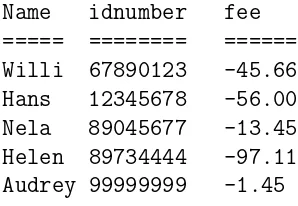
Example 6. The table is normally stored as a file, binary or text. In the following sixth example the table is given by

Name idnumber fee ===== ======== ====== Willi 67890123 -45.66 Hans 12345678 -56.00 Nela 89045677 -13.45 Helen 89734444 -97.11 Audrey 99999999 -1.45 ========================

Thus the table includes the name, the identity number and the outstanding fee. The table is stored as the text file mydata.txt

Willi 67890123 -45.66 Hans 12345678 -56.00 Nela 89045677 -13.45 Helen 89734444 -97.11 Audrey 99999999 -1.45

In our Java program we read the filemydata.txtand display the names and identity number und calculate the sum of the outstanding fees. We read each line using the method

String readLine()

in the class BufferedReader which reads a line of text. A line is considered to be terminated by any one of a line feed’\n’a carriage return’\r’or a carriage return followed immediately by a line feed. A String is returned containing the contents of the line, not including any line termination characters, or null if the end of the stream has been reached. a String.

(24)

// DataBase.java

import java.awt.*; import java.io.*; import java.util.*;

public class DataBase {

public static void main(String args[]) throws IOException {

int[] idnumber = new int[5]; String[] names = new String[5]; int i = 0;

String str;

double sum = 0.0;

FileInputStream fin = new FileInputStream("mydata.txt");

BufferedReader in = new BufferedReader(new InputStreamReader(fin));

while(!(null == (str = in.readLine()))) {

StringTokenizer tok = new StringTokenizer(str); String s1 = tok.nextToken();

names[i] = s1;

String s2 = tok.nextToken();

idnumber[i] = new Integer(s2).intValue();

String s3 = tok.nextToken();

double temp = new Double(s3).doubleValue(); sum += temp;

i++;

} // end while

in.close();

for(i=0; i < 5; i++) {

System.out.println("The name is: " + names[i] + " " + "The idnumber is: " + idnumber[i]); }

System.out.println("The sum is: " + sum); } // end main

(25)

Example 7. In a more advanced case we have a phone book with the phone number and the name. We want to insert names and phone numbers in the table, delete rows, write to the file, exit the manipulation of the database. We have the following commands:

?name find phone number

/name delete row with the given name !number name insert or update a row * list whole phonebook

= save to file (commit changes) # exit phonebook (database) For example, the command !34567 Cooper_Jack

inserts a row into the phonebook with the phone number 34567 and the name Cooper_Jack. To save it to the file phone.txt we have to apply the command =. In our C++ program we use the Standard Template Library (STL). Here less<T> is a function object that tests the truth or falsehood of some condition. If f is an object of class less<T>andx andy are objects of classT, then f(x,y)returns true if x < y and false otherwise.

// phone.cpp

#include <fstream> #include <iostream> #include <iomanip> #include <string> #include <map>

typedef map<string,long,less<string> > directype;

void ReadInput(directype& D) {

ifstream ifstr;

ifstr.open("phone.txt"); long nr;

string str; if(ifstr) {

cout << "Entries read from file phone.txt:\n"; for(;;)

(26)

ifstr >> nr;

ifstr.get(); // skip space getline(ifstr,str);

if(!ifstr) break;

cout << setw(9) << nr << " " << str << endl; D[str] = nr;

} }

ifstr.close(); }

void ShowCommands() {

cout <<

"Commands: ?name : find phone number\n" " /name : delete\n"

" !number name: insert (or update)\n" " * : list whole phonebook\n"

" = : save in file\n"

" # : exit" << endl; }

void ProcessCommands(directype& D) {

ofstream ofstr; long nr;

string str; char ch;

directype::iterator i; for(;;)

{

cin >> ch; // skip any whitespace and read ch switch(ch)

{

case’?’: case ’/’: getline(cin,str); i = D.find(str);

if(i == D.end()) cout << "Not found.\n"; else

if(ch == ’?’) cout << "Number: " << (*i).second << endl; else

D.erase(i); break;

(27)

if(cin.fail()) {

cout << "Usage: !number name\n"; cin.clear();

getline(cin,str); break;

}

cin.get();

getline(cin,str); D[str] = nr; break;

case ’*’:

for(i = D.begin(); i != D.end(); i++) cout << setw(9) << (*i).second << " "

<< (*i).first << endl; break;

case ’=’:

ofstr.open("phone.txt"); if(ofstr)

{

for(i = D.begin(); i != D.end(); i++) ofstr << setw(9) << (*i).second << " "

<< (*i).first << endl; ofstr.close();

}

else cout << "Cannot open output file.\n"; break;

case ’#’: break;

default: cout << "Use: * (list), ? (find), = (save), " "/ (delete), ! (insert), or # (exit), \n"; getline(cin,str);

break; }

if(ch == ’#’) break; }

}

int main() {

directype D; ReadInput(D); ShowCommands(); ProcessCommands(D); return 0;

(28)

Example 8. For Microprocessors we also use tables in particular lookup tables. As an example we consider the PIC 16F84 Microprocessor. We store a lookup table in the program memory. To access data in program memory, a table read operation must be performed. The table consists of a series of

RETLW K

statements. The command RETLWreturns with literal in W (W is the working register or accumulator for the PIC16F84). The 8-bit table constants are assigned to the literal K. The first instruction in the table

ADDWF PCL

computes the offset (counting from 0) to the table and consequently the program branches to a appropiate RETLW Kinstruction. The table contains the characters ’A’ ASCII table 65 dec 41 hex 01000001binary

’B’ ASCII table 66 dec 42 hex 01000010binary ’C’ ASCII table 67 dec 43 hex 01000011binary ’D’ ASCII table 68 dec 44 hex 01000100binary

Since we move 3 into W using the command MOVLW 3

and then add it to PCL (Program counter low) we select the character D which is ASCII 68 decimal and in binary 01000100. This bit string is moved to PORTB (out-put) and displayed.

The program counter PC in the PIC16F84 is 13-bits wide. The low 8-bits (PCL) are mapped in SRAM (static RAM) at location 02h and are directly readable and writeable. Let k be a label. Then

CALL k

calls a subroutine, where PC + 1 -> TOS(top of stack) and k -> PC.

(29)

PROCESSOR 16f84 INCLUDE "p16f84.inc"

ORG H’00’

Start

BSF STATUS, RP0 MOVLW B’11111111’ MOVWF PORTA

MOVLW B’00000000’ MOVWF PORTB

BCF STATUS, RPO

MOVLW 3 CALL Table

MOVWF PORTB

Table:

ADDWF PCL

RETLW ’A’ RETLW ’B’ RETLW ’C’ RETLW ’D’ ;

(30)

Example 9. For Web application of databases JavaScript is a good choice, since the program is embedded in the HTML file. Using a FORM the user enters the surname of the person and is provided with the complete information about the person (first name, street, and phone number).

<TITLE>Names Database</TITLE> <SCRIPT LANGUAGE="JavaScript">

Names = new Object() Names[0]=10

Names[1]="cooper" Names[2]="smith" Names[3]="jones" Names[4]="michaels" Names[5]="avery" Names[6]="baldwin"

Data = new Object()

function checkDatabase() {

var Found = false; // local variable

var Item = document.testform.customer.value.toLowerCase(); for(Count = 1; Count <= Names[0]; Count++)

{

if(Item == Names[Count]) {

Found = true;

var Ret = parser(Data[Count], "|"); var Temp = "";

for(i = 1; i <= Ret[0]; i++) {

Temp += Ret[i] + "\n"; }

alert(Temp); break;

(31)

}

if(!Found)

alert("Sorry, the name ’" + Item +"’ is not listed in the database.") } // end function checkDatabase()

function parser(InString,Sep) {

NumSeps=1;

for(Count=1; Count < InString.length; Count++) {

if(InString.charAt(Count)==Sep) NumSeps++;

}

parse = new Object();

Start=0; Count=1; ParseMark=0; LoopCtrl=1;

while(LoopCtrl==1) {

ParseMark = InString.indexOf(Sep,ParseMark); TestMark = ParseMark+0;

if((TestMark==0) || (TestMark==-1)) {

parse[Count]= InString.substring(Start,InString.length); LoopCtrl=0;

break; }

parse[Count] = InString.substring(Start,ParseMark); Start=ParseMark+1;

ParseMark=Start; Count++;

}

parse[0]=Count; return (parse);

} // end function parser </SCRIPT>

Enter the customer’s name, then click the "Find" button: <BR>

<INPUT TYPE="text" NAME="customer" VALUE="" onClick=0> <P> <INPUT TYPE="button" NAME="button" VALUE="Find"

onClick="checkDatabase()"> </FORM>

(32)

Example 10. The classJTable in Java provides a very flexible capability for cre-ating and displaying tables. The JTable class is another Swing component that does not have an AWT analog. The JTable class is used to display and edit regu-lar two-dimensional tables of cells. It allows tables to be constructed from arrays, vectors of objects, or from objects that implement the TableModel interface. The DefaultTableModel is a model implementation that uses a Vector of Vectors of Objects to store the cell values.

The following program gives an example. The table is given by

First Name Last Name Sport # of Years Vegetarian ========== ========= ============ ========== ==========

Mary Lea Snowboarding 5 no

Alison Humi Rowing 3 yes

Kathy Wally Tennis 2 no

Mark Andrews Boxing 10 no

Angela Lih Running 5 yes

===========================================================

// MyTable.java

import javax.swing.JTable;

import javax.swing.table.AbstractTableModel; import javax.swing.JScrollPane;

import javax.swing.JFrame;

import javax.swing.SwingUtilities; import javax.swing.JOptionPane; import java.awt.*;

import java.awt.event.*;

public class MyTable extends JFrame {

private boolean DEBUG = true;

public MyTable() {

super("MyTable");

MyTableModel myModel = new MyTableModel(); JTable table = new JTable(myModel);

table.setPreferredScrollableViewportSize(new Dimension(400,70));

(33)

getContentPane().add(scrollPane,BorderLayout.CENTER);

addWindowListener(new WindowAdapter() {

public void windowClosing(WindowEvent e) {

System.exit(0); }

});

} // end MyTable

class MyTableModel extends AbstractTableModel {

final String[] columnNames =

{ "First Name", "Last Name", "Sport", "# of Years", "Vegetarian" };

final Object[][] data = {

{ "Mary", "Lea", "Snowboarding", new Integer(5), new Boolean(false) }, { "Alison", "Humi", "Rowing", new Integer(3), new Boolean(true) }, { "Kathy", "Wally", "Tennis", new Integer(2), new Boolean(false) }, { "Mark", "Andrews", "Boxing", new Integer(10), new Boolean(false) }, { "Angela", "Lih", "Running", new Integer(5), new Boolean(true) } };

public int getColumnCount() { return columnNames.length; }

public int getRowCount() { return data.length; }

public String getColumnName(int col) { return columnNames[col]; }

public Object getValueAt(int row,int col) { return data[row][col]; }

public Class getColumnClass(int c) { return getValueAt(0,c).getClass(); }

public boolean isCellEditable(int row,int col) {

(34)

{ return true; } }

public void setValueAt(Object value,int row,int col) {

if(DEBUG) {

System.out.println("Setting value at " + row + "," + col + " to " + value + " (an instance of " + value.getClass() + ")"); }

if(data[0][col] instanceof Integer) {

try {

data[row][col] = new Integer((String) value); fireTableCellUpdated(row,col);

}

catch(NumberFormatException e) {

JOptionPane.showMessageDialog(MyTable.this, "The \"" + getColumnName(col)

+ "\" column accepts only integer values."); }

} else {

data[row][col] = value;

fireTableCellUpdated(row,col); }

if(DEBUG) {

System.out.println("New value of data:"); printDebugData();

}

private void printDebugData() {

(35)

for(int i=0; i < numRows; i++) {

System.out.print(" row " + i + "."); for(int j=0; j < numCols; j++)

{

System.out.print(" " + data[i][j]); }

System.out.println(); }

System.out.println("---"); }

}

MyTable frame = new MyTable(); frame.pack();

frame.setVisible(true); }

(36)

Example 11. An XML document is a database only in the strictest sense of the term. That is, it is a collection of data. In many ways, this makes it no different from any other file. All files contain data of some sort. As a database format, XML has some advantages. For example, it is self-describing (the markup describes the data), it is portable (Unicode), and it describes data in tree format. Every well-formed XML document is a tree.

A tree is a data structure composed of connected nodes beginning with a top node called the root. The root is connected to its child nodes, each of which is connected to zero or more children of its own, and so forth. Nodes that have no children of their own are called leaves. A diagram of a tree looks much like a genealogical descendant chart that lists the descendants of a single ancestor. The most use-ful property of a tree is that each node and its children also form a tree. Thus, a tree is a hierarchical structure of trees in which each tree is built out of samller trees. Fo the purpose of XSLT, elements, attributes, namespaces, processing instructions, and comments are counted as nodes. Furthermore, the root of the document must be distinguished from the root element. Thus, XSLT processors model an XML document as a tree that contains seven kinds of nodes:

1) the root 2) elements 3) text 4) attributes 5) namespaces

(37)

An example for the periodic table is given below (we only give the first two elements of the periodic table)

<?xml version="1.0"?>

<periodic_table> <atom>

<name> hydrogen </name> <symbol> H </symbol>

<atomic_number> 1 </atomic_number>

<atomic_weight> 1.00794 </atomic_weight> <atom_phase> gas </atom_phase>

</atom>

<atom>

<name> helium </name> <symbol> He </symbol>

<atomic_number> 2 </atomic_number> <atomic_weight> 4.0026 </atomic_weight> <atom_phase> gas </atom_phase>

</atom>

(38)

1.4

Table and Relation

The table is isomorphic to the mathematical relation, which puts the relational model of data onto firm theoretical foundations that allow the development of the-orems and proofs.

Consider two finite sets A and B. For example

A:={a, b}, B :={u, v, w, x}. The Cartesian product of the sets A and B is

A×B :={(a, u), (a, v), (a, w), (a, x), (b, u), (b, v), (b, w), (b, x)}.

Thus A×B contains 2·4 = 8 elements. A relation R is a subset of the Cartesian product of the sets on which it is defined. For example

R={(a, u), (a, x), (b, u), (b, v)}.

HereRis a subset ofA×B, which is another way of saying thatRis a set of couples (2-tuples) with the first element taken from the setA and the second element taken from the set B. As table we have

R == ==

a u

a x

b u

b v

======

The relational algebra (and any equivalent languges) is closed: algebraic operators take relations as operands and return relations as result, allowing the nesting of expressions to arbitrary depths.

The Cartesian product can be extended toS1×S2×. . .×SnofnsetsS₁,S₂, . . .Snis

the set of all orderedn-tuples (x1, x2, . . . , xn) in whichx₁ ∈S₁,x₂ ∈S₂, . . .xn∈Sn.

Since a relation is a set of tuples, we can apply the set theoretical operators UNION

INTERSECTION MINUS

TIMES (Cartesian product)

(39)

Let R be a relational scheme with a set of attributes X, where {A1, . . . , Ak} ⊆ X.

The projection of R onto {A1, . . . , Ak} is expressed by

SELECT DISTINCT A1, ... , Ak FROM R

Let R be a relational scheme with a set of attributes X, where A, B ∈ X. The selection of R with respect to condition A=a is expressed by

SELECT DISTINCT * FROM R WHERE A = a

Analogously, the selection with respect to condition A =B is expressed by SELECT DISTINCT * FROM R WHERE A = B

Let R and S be relational schemata with equal sets of attributes. The union of R and S is expressed by

SELECT DISTINCT * FROM R

UNION SELECT DISTINCT * FROM S

Analogously, the difference between R and S is expressed by SELECT DISTINCT * FROM R

EXCEPT SELECT DISTINCT * FROM S

Let R be a relational schema with attributes A1, . . . , An, B₁, . . . , Bm and S a

relational schema with attributes B1, . . . , Bm, C₁, . . . , Cl. Then the natural join

of R and S, which joins those tuples from R and S which have equal B-values, is expressed by

SELECT DISTINCT A1, ... , Am, R.B1, ... , R.Bm, C1, ... , Cl FROM R, S

WHERE R.B1 = S.B1 AND ... AND R.Bm = S.Bm

Since attributes from different relational schemata may have identical names, the dot-notation R.B is used to specify which occurrence of the respective attribute is meant. With respect to the natural join, of course, we could have used S.Bas well. The WHEREclause then explicitly states that tuples from the different relations must have identical values with respect to the shared attributes. A simpler formulation of the natural join, which is possible in SQL2, is

SELECT * FROM R NATURAL JOIN S

(40)

Chapter 2

Structured Query Language

2.1

Introduction

A database is a means of storing information in such a way that information can be retrievd from it. In simplest terms, a relational database is one that presents infor-mation in tables with rows and columns. A table is referred to as a relation, which explains the term relational database. A Database Management System (DBMS) handles the way data is stored, maintained, and retrieved. In the case of relational database, a Relational Database Management System (RDBMS) performs these tasks. DBMS as used here is a general term that includes RDBMS.

Structured Query Language (SQL) is a relational database language. Amongst other things the language consists of

select, insert, update, delete, query and protect data.

SQL allows users to access data in relational database mangement systems such as mySQL, Oracle, Sybase, Informix, DB2, Microsoft SQL Server, Access and others, by allowing users to describe the data the user wishes to see. Additionally SQL also allows users to define the data in a database and manipulate that data, for example update the data. SQL is the most widely used relational database language. Others are QBE and QUEL.

SQL is a nonprocedural language. We can use SQL to tell what data to retrieve or modify without telling it how to do its job. SQL does not provide any flow-of-control programming constructs, function definitions, do-loops, or if-then-else statements. However, for example Oracle provides procedural language extensions to SQL through a product called PL/SQL. ABAP/4 contains a subset of SQL (called Open SQL) that is an integral part of the language.

(41)

SQL provides a fixed set of datatypes in particular for strings of different length char(n), varchar(n), longvarchar(n)

We cannot define new datatypes. Unlike object-oriented programming language that allows to define a new datatype for a specific purpose, SQL forces us to choose from a given set of predefined datatypes when we create or modify a column. At the highest level, SQL statements can be broadly categorized as follows into three types:

Data Manipulation Language (DML), which retrieves or modifies data Data Definition Language (DDL), which defines the structure of the data

Data Control Language (DCL), which defines the privileges granted to database users.

The category of DML contains four basic statements:

SELECT, which retrieves rows from a table. The SELECT statement specifies which columns to include in the result set. The vast majority of the SQL commands used in applications are SELECT statements.

INSERT, which adds rows to a table. INSERT is used to populate a newly-created table or to add a new row (or rows) to an already-existing table.

UPDATE, which modifies existing rows in a table. In other words it changes an exist-ing value in a column of a table.

DELETE, which removes a specified row or a set of rows from a table.

(42)

The most common DDL commands are:

CREATE TABLE, creates a table with the column names the user provides. The user also needs to specify the data type for each column. Unfortunately, data types vary slighly from one RDBMS to another, so that user might need metadata to estab-lish the data types used for a particular database. The command CREATE TABLE is normally used less often than the data manipulation commands because a table is created only once, whereas inserting and deleting rows or changing individual values generally occurs more frequently.

DROP TABLE, deletes all rows and removes the table definition from the database.

ALTER TABLE, adds or removes a column from a table. This command is used in connection with ADD,MODIFY and DROP.

For most systems (for example mySQL, Oracle), every SQL statement is terminated by a semicolon. An SQL statement can be entered on one line or split accross sev-eral lines for clarity. Most of the examples given here are split into readable portions. For most systems SQL is not case sensitive. We can mix uppercase and lowercase when referencing SQL keywords (such as SELECT and INSERT), tables names, and column names. However, case does matter when referring to the contents of a col-umn.

Before we can create a table we have to create a database. For example in mySQL we have the command

CREATE DATABASE [IF NOT EXISTS] db_name;

(43)

2.2

Integrity Rules

Relational tables follow certain integrity rules to ensure that the data they contain stay accurate and are always accessible.

First, the rows in a relational table should all be distinct. If, there are duplicates rows, there can be problems resolving which of two possible selections is the correct one. For most DBMSs, the user can specify that duplicate rows are not allowed, and if that is done, the DBMS will prevent the addition of any rows that duplicates an existing row.

A second integrity rule is that column values cannot be repeating groups or arrays. A third aspect of data integrity involves the concept of a null value. A database has to take care of situations where data may not be available: a null value indicates that a value is missing. It does not equate to a blank or zero. A blank is considered equal to another blank, a zero is equal to another zero, but two null values are not considered equal.

When each row in a table is different, it is possible to use one or more columns to identify a particular row. This unique column or group of columns is called a primary key. Any column that is part of a primary key cannot be null; if it were, the primary key containing it would no longer be a complete identifier. This rule is referred to as entity integrity.

Thus some of an entity’s attributes uniquely identify each row in that entity. This set of attributes is called the primary key.

From a managerial design perspective, it is a good idea to assume that the RDBMS in use does not enforce referential integrity. Further, it is a good idea to assume that the programmer/analyst with whom we are working is not necessarily going to design the system to enforce referential integrity. It is our responsibility to define procedures that enforce referential integrity.

(44)

2.3

SQL Commands

2.3.1

Introduction

SQL (Structered Query Language) is a language designed to be used with relational databases. There is a set of basic SQL commands that is considered standard and is used by all RDBMSs. For example, all RDBMSs use the SELECT statement. In this section we list the SQL commands and give a number of examples. In the following we assume the following tables are given. The name of the tables are Employees and Cars.

table: Employees

=========== ========== ========= ============= ========== Employee_No First_Name Last_Name Date_of_Birth Car_Number =========== ========== ========= ============= ==========

10001 John Smith 28-AUG-1943 5

10083 Axel Sharma 24-DEC-1954 null

10120 Jonas Goldberg 01-JAN-1956 null

10005 Florence Wojokowski 04-JUL-1971 12

10099 Sean Smith 21-SEP-1966 null

10035 Liz Yamaguchi 24-DEC-1967 null

==============================================================

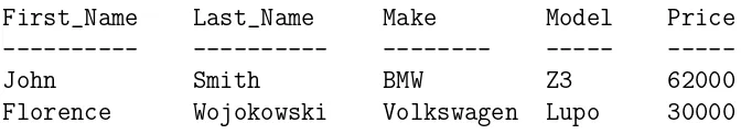
In this table of employees, there are five columns: Employee_No, First_Name, Last_Name,Date_of_Birth, andCar_Number. There are six rows, each representing a different employee. The primary key for this table would generally be the employee number because each one is guaranteed to be different. A number is more efficient than a string for making comparisons. It would also be possible to use First_Name and Last_Name together because the combination of the two also identifies just one row in our sample database. Using the last name alone would not work because there are two employees with the last name ofSmith. In the particular case the first name are all different, so one would conceivably use that column as a primary key, but when we add new names to the table the same first name could appear twice. If we would use the first name as the primary key and add a new employee with the name Sean Connery to the table the RDMS will not allow his name to be added. table: Cars

========== ======== ======= ===== ======

Car_Number Make Model Year Price

========== ======== ======= ===== ======

5 BMW Z3 1999 62000

12 Volkswagen Lupo 2000 30000

(45)

2.3.2

Aggregate Function

SQL system allow five aggregate functions, SUM,AVG,MAX,MIN, andCOUNT. They are called aggregate functions because they summarize the result of a query.

SUM() gives the total of all the rows, satisfying any conditions, of the given column, where the given column is numeric.

AVG() gives the average (arithmetic mean) of the given column (does floating point division)

MAX() gives the largest number in the selected column MIN() gives the smallest number in the selected column COUNT(*) gives the number of rows satisfying the conditions

2.3.3

Arithmetic Operators

The arithmetic operators used in SQL are similar to those in C.

Description Operator

=========== ========

Addition +

Subtraction

-Multiplication *

Division /

There are six relational operators in SQL.

Less than <

Less than or equal to <=

Greater than >

Greater than or equal to >=

Equal to =

Not equal to !=

2.3.4

Logical Operators

(46)

2.3.5

SELECT Statement

The SELECT statement, also called a query, is used to get information from a table. It specifies one or more column headings, one or more tables from which to select, and some criteria for selection.

Example 1. We want to get all columns and rows from the table Cars. SELECT Car_Number, Make, Model, Year, Price

FROM Cars;

This displays the whole table. To get all columns and rows of a table without typing all columns we can use *. Thus

SELECT * FROM Cars;

The WHEREclause (conditional selection) is used to specify that only certain rows of the table are displayed, based on the criteria described in that WHERE clause. Example 2. We select from table Employee theLast_Name and Car_Numberwhen the First_Name isSean

SELECT Last_Name, Car_Number FROM Employees

WHERE First_Name = ’Sean’;

The result set (output) is Last_Name Car_Number ---

---Smith null

---Example 3. The command SELECT Make

FROM Cars

WHERE Price > 60000;

gives the output Make

(47)

----Example 4. The command

SELECT First_Name, Last_Name FROM Employees

WHERE Car_Number IS NOT NULL;

gives the output

First_Name Last_Name ---

---John Smith

Florence Wojokowski

---Example 5. An application of the arithmetic operation + is as follows

SELECT Model, Price + 5000 FROM Cars;

The output is

Model Price + 5000 ---

---Z3 67000

Lupo 35000

---Example 6. An application of the logicalAND is SELECT First_Name, Last_Name

FROM Employees

WHERE Employee_Number < 10010 AND Car_Number IS NULL;

The result set is empty. The wildcards are

% zero or more characters

and

_ only one character

(48)

SELECT First_Name, Last_Name FROM Employees

WHERE Last_Name LIKE ’Smit%’;

ThenSmit andSmithmatch, but also Smithlingetc. This means% stands for plus zero or more additional characters. The result set is

---John Smith

Sean Smith

---Example 8. Consider the command SELECT First_Name, Last_Name FROM Employees

WHERE Last_Name LIKE ’S_ith’;

The other wildcard used in LIKEclauses is an underbar_, which stands for any one character. It matches Smith, but also Snith, Skith etc.

The result set is

---John Smith

Sean Smith

---Example 9. The query SELECT COUNT(*) FROM Employees

WHERE Car_Number IS NULL;

counts the number of employees which have no car.

Example 10. The IN operator has to be understood in the set theoretical sense. For example

SELECT First_Name FROM Employees

WHERE Last_Name IN (’Smith’, ’Sharma’);

(49)

Example 11. Using the BETWEEN operator we can give a numerical range. For example

SELECT Model FROM Cars

WHERE Price NOT BETWEEN 30000 AND 50000;

Example 12. To sort data we use the ORDER BY clause. It sorts rows on the basis of columns. TheORDER BYclause is optional. By default the database system orders the rows in ascending order.

SELECT Last_Name, First_Name, Date_of_Birth FROM Employees

ORDER BY Last_Name, First_Name;

To order the rows in descending order, we must add the keyword DESC after the column name.

A SELECT statement can be nested inside of another SELECT statement which is nested of another SELECT and so on. When a SELECT is nested it is refered to as a subquery clause. An example is

SELECT first_name AS name, last_name AS surname FROM Employees

WHERE car_number IN

(SELECT DISTINCT car_number FROM cars WHERE car_number > 4);

TheDISTINCTpredicate is used to omit duplicate values just in a field. For example, if we have the last name Smith repeated numerous times in the table Employees then the code

SELECT DISTINCT Last_Name FROM Employees;

(50)

2.3.6

INSERT Command

The INSERT command adds rows to a table. We supply literal values or expressions to be stored as rows in the table. The term INSERT leads some new SQL users to think that they can control where a row is inserted in a table. Recall that a large reason for the use of relational databases is the logical data independence they offer - in other words, a table has no implied ordering. A newly inserted row simply goes into a table at an arbitrary location.

The INSERT commands takes the form INSERT INTO table_name

[(column_name[,column_name]...[,column_name])] VALUES

(column_value[,column_value]...[,column_value])

where

table_name table in which to insert the row column_name column belonging to table_name column_value literal value or an expression

whose type matches the corresponding column_name

Notice that the number of columns in the list of column names must match the num-ber of literal values or expressions that appear in the parentheses after the keyword VALUES. If it does not match the database system returns an error message. The column and value datatype must match. Inserting an alphanumeric string into a numeric column, for example, does not make any sense. Each column value supplied in an INSERT command must be one of the following:

1) A null, 2) A literal value, such as 3 or ’Swiss’.

An expression containing operators and functions, such asSUBSTR(Last_Name,1,4). We notice that the column list is an optional element. If we do not specify the column names, the database system uses all the columns. In addition, the column order that the database system uses is the order in which the columns were specified when the table was created.

Example. As an example we insert a new row into the table Cars. INSERT INTO Cars

(Car_Number, Make, Model, Year, Price) VALUES

(51)

2.3.7

DELETE Command

The DELETE statement removes rows from a table. We do not need to know the physical ordering of the rows in a table to perform a DELETE. The database system uses the criteria in theWHEREclause to determine which rows to delete. The database engine determines the internal location of the rows.

The DELETE commamd has the simplest syntax of the four DML statements DELETE FROM table_name

[WHERE condition]

The variables are defined as follows

table_name is the table to be updated condition is a valid SQL condition

Example 1. In the table Cars we delete one row with the Make BMW. DELETE FROM Cars

WHERE Make = ’BMW’;

Example 2.

DELETE FROM Employees WHERE Car_Number IS NULL;

If we want to delete all rows the DELETE statement is quite inefficient. The TRUNCATE TABLE table_name

deletes rows much faster than the DELETE command does. Notice that a TRUNCATE TABLE

(52)

2.3.8

UPDATE Command

If we want to modify existing data in an SQL database, we need to use the UPDATE command. With this statement, we can update zero or more rows in a table. The UPDATE statement has the following syntax.

UPDATE table_name

SET column_name = expression [, column = expression] ... [, column = expression] [WHERE condition]

The variables are defined as follows. table_name table to be updated

column_name column in the table being updated expression valid SQL expression

condition valid SQL condition

Example 1.

UPDATE Cars

SET Price = 70000 WHERE Make = ’BMW’;

Example 2.

UPDATE Cars

(53)

2.3.9

CREATE TABLE Command

To generate a table we use the CREATE TABLE statement. Each table must have a unique name. A table name cannot be an SQL reserved word. A table name should be descriptive. Within a single table, a column name must be unique. A column name cannot be an SQL reserved word. We also have to provide the datatype for each column. Furthermore, we can supply the primary key constraints and the NOT NULL constraint.

The CREATE TABLE syntax is CREATE TABLE table_name (

column_name1 data_type [NOT NULL], ...

column_nameN datatype [NOT NULL], [Constraint constraint_name]

[Primary key (column_nameA, column_nameB, ... column_nameN)]);

The variables are defined as follows table_name name for the table

column_name1 through column_nameN valid colun names datatype valid datatype specification

constraint_name optional name that identifies the primary key constraint

column_nameA through column_nameN table’s columns that compose the primary key

Constraints include the following possibilities: NULL or NOT NULL, UNIQUE enforces that no two rows will have the same values for this column, PRIMARY KEY tells the database that this column is the primary key.

Example 1. Oracle style (for mySQL replace NUMBER(8) by INT for Integers (4 bytes)).

CREATE TABLE Square (x NUMBER(6),

x2 NUMBER(6));

Example 2. Oracle style (for mySQL replace VARCHAR2(10)by VARCHAR(10)and NUMBER(5) by INT).

CREATE TABLE Employees

(EMPLOYEE_NUMBER NUMBER(5) NOT NULL, FIRST_NAME VARCHAR2(10),

(54)

We can also write our create statement in a SQL file. Then we read this file (Oracle style).

-- exam1.sql

DROP TABLE Employees; DROP TABLE Cars;

(EMPLOYEE_NUMBER NUMBER(5) NOT NULL, FIRST_NAME VARCHAR2(10),

LAST_NAME VARCHAR2(10), DATE_OF_BIRTH VARCHAR2(10), CAR_NUMBER NUMBER(5));

INSERT INTO Employees VALUES

(10001,’John’,’Smith’,’28-AUG-43’,5); INSERT INTO Employees VALUES

(10083,’Arvid’,’Sharma’,’24-NOV-54’,null); INSERT INTO Employees VALUES

(10035,’Sean’,’Washington’,’22-FEB-81’,12);

CREATE TABLE Cars

(CAR_NUMBER NUMBER(2), MAKE VARCHAR2(14), MODEL VARCHAR2(14), YEAR NUMBER(4));

INSERT INTO Cars VALUES (5,’BMW’,’Z3’,1998); INSERT INTO Cars VALUES

(12,’VW’,’POLO’,1999);

In mySQL the command

LOAD DATA INFILE ’file_name.txt’ INTO TABLE tbl_name

(55)

In the following SQL file we also include a primary key and foreign key (Oracle style).

-- exam2.sql

DROP TABLE Employees; DROP TABLE Cars;

CREATE TABLE Cars

(CAR_NUMBER NUMBER(5), MAKE VARCHAR2(14), MODEL VARCHAR2(14), YEAR NUMBER (4), CONSTRAINT PK_CARS Primary Key (CAR_NUMBER));

(EMPLOYEE_NUMBER NUMBER(5) NOT NULL, FIRST_NAME VARCHAR2(20),

LAST_NAME VARCHAR2(20), DATE_OF_BIRTH VARCHAR2(10), CAR_NUMBER NUMBER (5), CONSTRAINT PK_EMPLOYEES

Primary Key (EMPLOYEE_NUMBER,CAR_NUMBER), CONSTRAINT FK_EMPLOYEES_CAR_NUMBER

Foreign Key (CAR_NUMBER) REFERENCES Cars (CAR_NUMBER));

INSERT INTO Cars VALUES (5,’BMW’,’Z3’,1998); INSERT INTO Cars VALUES

(12,’VW’,’Polo’,1999); INSERT INTO Cars VALUES

(6,’MERCEDES’,’BENZ’,1999);

INSERT INTO Employees VALUES

(10001,’John’,’Smith’,’28-Aug-43’,5); INSERT INTO Employees VALUES

(10083,’Arvid’,’Sharma’,’24-Nov-54’,6); INSERT INTO Employees VALUES

(56)

2.3.10

DROP TABLE Command

The SQL DROP TABLE command is used if we decide that a base relation in the database is not needed any longer. We can then delete the relation and its definitions using theDROP TABLEcommand. This also removes a tuple from theSYSTABLESand system catalog table. This meansDROP TABLEdeletes all rows and removes the table definition from the database.

The syntax is as follows DROP TABLE table_name;

Example.

DROP TABLE Cars;

(57)

2.3.11

ALTER TABLE Command

Sometimes it is necessary to modify a table’s definition. TheALTER TABLEstatement serves this purpose. This statement changes the structure of a table, not its con-tents. Using ALTER TABLE, the changes we can make to a table include the following 1) Adding a new column to an existing table

2) Increasing or decreasing the width of an existing column

3) Changing an existing column from mandatory to optional or vice versa 4) Specifying a default value for an existing column

5) Specifying other constraints for an existing column

Here are the four basic forms of the ALTER TABLE statement: ALTER TABLE table_name

ADD (column_specification | constraint , ... column_specification | constraint);

ALTER TABLE table_name

MODIFY (column_specification | constraint , ... column_specification | constraint);

ALTER TABLE table_name DROP PRIMARY KEY;

ALTER TABLE table_name DROP CONSTRAINT constraint;

The variables are defined as follows: table_name name of the table

column_specification valid specification for a column (column name and datatype)

constraint column or table constraint

The first form of the statement is used for adding a column, the primary key, or a foreign key to a table. The second form of the statement is used to modify an ex-isting column. Among other things, we can increase a column’s width or transform it from mandatory to optional. The third and fourth forms of the ALTER TABLE statement are used for dropping a table’s primary key and other constraints. Example.

(58)

2.4

Set Operators

In this section we consider the set operators in the SELECT statement. The SQL language is a partial implementation of the model as envisioned by Codd, the father of relational databases. As part of that implementation SQL provides three set operators

INTERSECT, UNION, MINUS

The mathematical symbols are ∩, ∪, \. Let A and B be two sets. The definitions are

A∩B :={x∈A and x∈B}

A∪B :={x∈A or x∈B}

A\B :={x∈A x /∈B}.

The symmetric difference ∆ of the sets A and B is defined as A△B := (A∪B)\(A∩B). Example. Let

A={"Olten", "Johannesburg", "Singapore"}

B ={"Johannesburg","Stoeckli"}. Then

A∩B ={"Johannesburg"}

A∪B ={"Olten", "Johannesburg", "Singapore", "Stoeckli"}

A\B ={"Olten", "Singapore"}

If the set is finite with n-elements, then the number of subsets (including the empty set and the set itself) is 2n

(59)

The INTERSECT Operator

The INTERSECT operator returns the rows that are common between two sets of rows. The syntax for using the INTERSECT operator is

SELECT stmt1 INTERSECT SELECT stmt2 [ORDER BY clause]

The variables are defined as follows: SELECT stmt1

and

SELECT stmt2

are valid SELECT statements. The ORDER BYclause references the columns by num-ber rather than by name.

Requirements and considerations for using the INTERSECT operator are:

The two SELECT statements may not contain anORDER BY clause. However, we can order the result of the entire INTERSECT operation.

The number of columns retrieved by SELECT stmt1 must be equal to the number of columns retrieved by SELECT stmt2.

The datatypes of the columns retrieved bySELECT stmt1must match the datatypes of the columns retrieved by SELECT stmt2.

(60)

The UNION Operator

To combine the rows from similar tables or produce a report or to create a table for analysis we apply the UNION operator. The syntax is

SELECT stmt1 UNION

SELECT stmt2 [ORDER BY clause]

The variables are defined as follows SELECT stmt1

and

SELECT stmt2

are valid SELECT statements. The ORDER BYclause references the columns by num-ber rather than by name.

The MINUS Operator

The syntax is SELECT stmt1 MINUS

SELECT stmt2 [ORDER BY clause]

The variables are defined as follows SELECT stmt1

and

SELECT stmt2

(61)

Both C++ using the STL with the classsetand Java with the classTreeSetallow set-theoretical operations. We can find the union, intersection and difference of two finite sets. We can also get the cardinality of the finite set (i.e. the number of elements). Furthermore, we can find out whether a finite set is a subset of another finite set and whether a finite set contains a certain element.

In C++ the class set is a sorted associative container that stores objects of type Key. The class set is a simple associative container, meaning that its value type, as well as its key type, is key. It is also a unique associative container meaning that no two elements are the same. The C++ class set is suited for the set algorithms includes,

set_union, set_intersection,

set_difference, set_symmetric_difference

The reason for this is twofold. First, the set algorithms require their arguments to be sorted ranges, and, since the C++ class set is a sorted associative container, their elements are always sorted in ascending order. Second, the output range of these algorithms is always sorted, and inserting a sorted range into a set is a fast operation. The class sethas the important property that inserting a new element into a set does not invalidate iterators that point to existing elements. Erasing an element from a set also does not invalidate any iterator, except of course, for iterators that actually point to the element that is being erased. Other functions in the C++ class setare

bool empty()

which returns true if the container is empty, int size()

which returns the number of elements in the container. The following program shows an application of this class. // setstl.cpp

#include <iostream> #include <set>

#include <algorithm> #include <string.h>

(62)

bool operator() (const char* s1,const char* s2) const {

return strcmp(s1,s2) < 0; }

};

int main() {

const int N = 3;

const char* a[N] = { "Steeb", "C++", "80.00" }; const char* b[N] = { "Solms", "Java", "80.00" };

set<const char*,ltstr> S1(a,a+N); set<const char*,ltstr> S2(b,b+N); set<const char*,ltstr> S3;

cout << "union of the sets S1 and S2: " << endl; set_union(S1.begin(),S1.end(),S2.begin(),S2.end(),

ostream_iterator<const char*>(cout," "),ltstr()); cout << endl;

cout << "intersection of sets S1 and S2: " << endl;

set_intersection(S1.begin(),S1.end(),S2.begin(),S2.end(),

ostream_iterator<const char*>(cout," "),ltstr()); cout << endl;

set_difference(S1.begin(),S1.end(),S2.begin(),S2.end(), inserter(S3,S3.begin()),ltstr());

cout << "Set S3 difference of S1 and S2: " << endl;

copy(S3.begin(),S3.end(),ostream_iterator<const char*>(cout," ")); cout << endl;

// S2 subset of S1 ?

bool b1 = includes(S1.begin(),S1.end(),S2.begin(),S2.end(),ltstr()); cout << "b1 = " << b1 << endl;

// S4 subset of S2 ?

const char* c[1] = { "Solms" }; set<const char*,ltstr> S4(c,c+1);

bool b2 = includes(S2.begin(),S2.end(),S4.begin(),S4.end(),ltstr()); cout << "b2 = " << b2;

(63)

In Java the interface Set is a Collection that cannot contain duplicates elements. The interface Set models the mathematical set abstraction. The Set interface extends Collection and contains no methods other than those inherited from Collection. It adds the restriction that duplicate elements are prohibited. The JDK contains two general-purpose Setimplementations. The class HashSetstores its elements in a hash table. The class TreeSet stores its elements in a red-black tree. This guarantees the order of iteration.

The following program shows an application of the TreeSetclass.

// SetOper.java

import java.util.*;

public class SetOper {

String[] A = { "Steeb", "C++", "80.