Nanoseostetun epoksin valmistus ja karakterisointi

(1)

EEVA HYKKÖ

MANUFACTURING AND CHARACTERIZATION OF NANOFILLED

EPOXY

Master of Science Thesis

Examiners: Professor Pentti Järvelä And Docent Mikael Skrifvars

Examiners and Topic Approved in The Automation, Mechanical and Materials Council Meeting on 6th of June 2012

(2)

ii

ABSTRACT

TAMPERE UNIVERSITY OF TECHNOLOGY Master’s Degree Programme in Materials Science

HYKKÖ, EEVA: Manufacturing and characterization of nanofilled epoxy Master of Science Thesis, 71 pages, 7 appended pages

May 2013

Major subject: Polymeric materials

Examiners: Professor Pentti Järvelä and Docent Mikael Skrifvars

Key words: nanocomposites, epoxy, nano-SiO2, silicon dioxide, nanoclay, multi-walled carbon nanotubes

Nanocomposites are a new field in the polymer industry offering improved mechanical, thermal, electrical and optical properties with low filler content. Nanocomposites have a huge potential in many applications, but the preparation methods are still under investigation. This is due to the tendency of nanoparticles to form large clusters during manufacturing due to their small size and high surface energy. Improved properties in composites cannot be achieved if the nanofiller dispersion is poor.

The scope of this study was to successfully manufacture epoxy composites with uniform nanofiller dispersion. Furthermore, the mechanical, thermal and rheological properties of the prepared samples were examined. Nanosized silicon dioxide (SiO2),

organoclay and multi-walled carbon nanotubes (MWCNT) were incorporated into the epoxy resin by high shear mixing. Samples were prepared by moulding and the curing with a hardener was performed at elevated temperature.

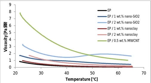
Some difficulties were observed during manufacturing. A notable amount of air bubbles was formed on the resin during the mixing of the nanofillers and their removal slowed down the manufacturing process. Furthermore, viscosity of the nanofilled resin was strongly affected by the nanoparticles limiting the preparation of higher filler loadings. Small amounts (0.5 wt.%) of MWCNTs increased the viscosity of the resin significantly. In case of nano-SiO2 and nanoclay, concentration of 2 wt.% increased the

viscosity so that the air bubble removal was extremely slow. Furthermore, the mixing of sample with 4 wt.% of nano-SiO2 was not possible anymore with the high shear mixer

due to the markedly increased viscosity.

Improved properties in mechanical and thermal tests were not totally achieved. Scanning electron microscope (SEM) and field emission scanning electron microscope (FESEM) images indicated that the samples contained agglomerated nanoparticles indicating that the mixing may not have been effective enough.

Difficulties during manufacturing and the poor dispersion in the final composites require further research in terms of more effective preparation methods and matrix/filler compatibility. Other processing methods (such as ultrasonication or using solvents) in addition to high shear mixing are needed to achieve proper dispersion.

(3)

iii

TIIVISTELMÄ

TAMPEREEN TEKNILLINEN YLIOPISTO Materiaalitekniikan koulutusohjelma

HYKKÖ, EEVA: Nanoseostetun epoksin valmistus ja karakterisointi Diplomityö, 71 sivua, 7 liitesivua

Toukokuu 2013

Pääaine:Tekniset polymeerimateriaalit

Tarkastajat:Professori Pentti Järvelä and Dosentti Mikael Skrifvars

Avainsanat: Nanokomposiitti, epoksi, nano-SiO2, nanosavi, moniseinämäinen hiilinanoputki

Nanokomposiitit ovat yksi uusimpia materiaaleja polymeeriteollisuudessa, joilla voidaan saavuttaa parannuksia mekaanisissa, termisissä, sähköisissä ja optisissa ominaisuuksissa varsin pienillä täyteainepitoisuuksilla. Nanokomposiittien valmistus on kuitenkin edelleen hyvin haasteellista, sillä nanokokoiset partikkelit muodostavat erittäin helposti agglomeraatteja. Jotta nanokomposiittien hyvät ominaisuudet voidaan saavuttaa, täytyy nanotäyteaineen olla tasaisesti dispergoitunut matriisiin.

Tämän työn tavoitteena oli valmistaa epoksinanokomposiitteja käyttäen eri nanotäyteaineita ja testata lopullisten nanokomposiittien mekaanisia, termisiä ja reologisia ominaisuuksia. Nanokokoista silikaa (SiO2), nanosavea ja moniseinämäisiä

hiilinanoputkia (MWCNT) sekoitettiin epoksimatriisiin korkealla leikkausnopeudella. Näytteet valmistettiin valamalla sekoitettu hartsi ja kovettaja muotteihin ja kovettamalla ne korotetussa lämpötilassa.

Nanokomposiittien valmistuksen aikana ilmeni joitakin hankaluuksia. Sekoituksen aikana hartsiin muodostui ilmakuplia, joiden poistaminen hidasti merkittävästi valmistusprosessia. Lisäksi nanotäyteaineet kasvattivat selvästi hartsin viskositeettia, mikä rajoitti korkeampien täyteainepitoisuuksien valmistusta. Puolen painoprosentin MWCNT-pitoisuus kasvatti viskositeettia huomattavasti enemmän kuin muut nanotäyteaineet. Viskositeetin nousu näytteissä joissa oli kaksi painoprosenttia nano-SiO2:a tai nanosavea hidasti merkittävästi ilmakuplien poistoa. Neljä painoprosenttia

nano-SiO2:a nosti viskositeettia niin paljon että mekaaninen sekoitus ei enää ollut

mahdollista.

Parannuksia mekaanisissa ja termisissä ominaisuuksissa ei täysin saavutettu. Elektronimikroskooppikuvat paljastivat, että näytteet sisälsivät agglomeroituneita nanopartikkeleita osoittaen, että nanotäyteaineiden dispersio ei ollut riittävä toivottujen ominaisuuksien saavuttamiseksi.

Haasteet valmistusvaiheessa ja nanotäyteaineiden heikko dispersio osoittavat, että lisätutkimukselle on tarvetta nanokomposiittien valmistusmenetelmien ja raaka-aineiden yhteensopivuuden parantamiseksi. Muita prosessointimenetelmiä (kuten ultraäänisekoitusta tai liuottimen käyttöä) on tarpeen yhdistää korkean leikkausnopeuden sekoittamiseen tarvittavan dispersion aikaansaamiseksi.

(4)

iv

PREFACE

This thesis was done at Tampere University of Technology for the Plastics and Elastomers Department from April 2012 to May 2013.

I would like to specially thank my supervisors Professor Pentti Järvelä and Docent Mikael Skrifvars for giving me this opportunity, for their advices and guidance throughout the work and for evaluating my thesis. I would also like to thank Egidija Rainosalo for her advices and help.

I am very grateful for Reija Suihkonen for the invaluable guidance with the nanocomposite preparation and for her assistance with the writing work.

I would also like to thank Professor Jyrki Vuorinen for providing me the facilities and work safety to work with the nanoparticles, Olli Orell for the help in the tensile and fracture toughness tests, Seppo Syrjälä for the rheology measurements, Sinikka Pohjonen for the thermal analysis tests and the SEM-imaging, Kosti Rämö for the thermal analysis tests and help with the laboratory work, Merja Ritola also for the SEM-imaging, Jarmo Laakso and the Material’s department for the FESEM SEM-imaging, and everyone else who gave me advice, and the whole Plastics and Elastomers department for the inspiring environment.

I also want to thank my family and friends for the support during my studying, and especially my parents for the encouragement during the intense work period with the thesis.

Tampere 10.5.2013

(5)

v

ABBREVIATIONS AND NOTATIONS

Ø Diameter Strain Stress ohm a Crack length A Area Ag Silver Au Gold B Thickness CNT Carbon nanotube

CVD Catalytic chemical vapour deposition

d Diameter

DMA Dynamic mechanical analysis DSC Differential scanning calorimetry

E Young’s modulus

E’ Storage modulus

E’’ Loss modulus

EP Epoxy

EPDM Ethylene propylene diene monomer EVA Ethylene vinyl acetate

F Force

Fe3O4 Iron oxide

FESEM Field emission scanning electron microscopy

I Current

Kic Critical stress intensity factor

MWCNT Multi-walled carbon nanotubes

min minutes

n rotating speed

N2 Nitrogen

NBR Nitrile butadiene rubber

NR Natural rubber nm Nanometer O2 Oxygen Pa Pascal PA Polyamide PC Polycarbonate

PE-HD High-density polyethylene

PEI Polyetherimide

(8)

viii

PP Polypropylene

PQ Critical load for crack propagation

PS Polystyrene

PU Polyurethane

PVC Polyvinyl chloride

Rs Surface resistivity

Rv Volume resistivity

rpm Revolution per minute

SBR Styrene-butadiene rubber SEM Scanning electron microscopy SiO2 Silicon dioxide, silica

t Thickness of the sample

TEM Transmission electron microscopy Tg Glass transition temperature

TGA Thermogravimetric analysis TiO2 Titanium dioxide

TPO Thermoplastic olefin

U Voltage

v Circumference velocity

W Width

(9)

1

1 INTRODUCTION

Nanoparticles, having one dimension less than 100 nm [1], have gained increased interest during the past few years. This is due to their novel properties and high potential for many applications, such as in biology, medicine, electronics, chemical processes and high-strength materials. [2] Polymeric nanocomposites are one of the newest polymeric materials that are discovered and developed. [3] Nanocomposites offer improved mechanical, thermal, electrical and optical properties compared to conventional composites. [1] This is due to the large aspect ratio and high specific surface area of the nanoparticles, which enable greater interaction between the fillers and the matrix. [4] Applications of the nanocomposites include aerospace, coatings, electronics, sports goods and automotive industries. [5]

Polymer nanocomposites consist of polymer matrix and nanofillers. Studies have been made widely in thermoplastics, for example PA, PP, PS, PVC [6], PE-HD [7], EVA [8], PET [9], PC, TPOs, and PEI [10]. Also thermosets, such as epoxy [1], vinyl ester [5], phenol [11], cyanate ester [12], unsaturated polyester and polyimide [13] and elastomers, for example NR, SBR, PU, silicone [14], EPDM and NBR [15] have been studied.

Mixing of the nanosized fillers on the polymer can improve its mechanical properties due to the high specific surface area of the particles that can enhance the stress transfer from matrix to the nanoparticles. Other properties like dimensional stability, flame retardancy, gas barrier properties and corrosion resistance can also be improved. The filler-matrix interface determines the degree of interaction between the filler and the matrix and therefore proper dispersion and the interfacial interactions are needed for achieving the desired properties. [16]

Because of the very small particle size, the manufacturing process and the final properties of the nanocomposite are very difficult to control. [1] Nanoparticles have a high tendency to form agglomerates, where the particles are stuck together by adhesive forces. [4] In addition to the large surface area, adhesive forces tend to increase when the particle size decreases. [17] The stacked fillers are not in nanoscale anymore and will behave like conventional fillers losing the advantages of the small particle size. [4] Therefore, preparation of the true nanocomposite is crucial and it has become a technological challenge in materials science. [1] The right preparation methods for the nanoparticles and the proper dispersion techniques are still under research. Furthermore, high cost of some nanofillers, especially carbon nanotubes, has also restricted the usage of nanofillers in a large scale. When the nanocomposite technologies develop, the nanofiller market will increase and the costs will reduce. [4]

(10)

2

In this work, nanocomposites with different nanoparticles were prepared and the samples were characterized with different methods. Three different nanofillers were used to prepare epoxy nanocomposites with epoxy resin: 1 and 2 wt.% of nano-SiO2, 1

and 2 wt.% of nanoclay and 0.5 wt.% of MWCNTs. High shear mixing was used to disperse the nanoparticles into the matrix. Interaction between the fillers and the matrix and the level of dispersion were analyzed by the test results that included viscosity measurements, tensile tests, fracture toughness tests and thermal analysis methods. The samples were also investigated by scanning electron microscopes.

The main goal of this work was to investigate the behaviour of the nanofillers with the epoxy resin and to examine the potential of the high shear mixing as an option for the nanocomposite preparation. These results will give more information about thermoset nanocomposite preparation and lay the groundwork for further research.

(11)

3

2 POLYMER NANOCOMPOSITES

2.1 General

Polymer nanocomposite is a structure that consists of two interacting phases, a polymer matrix and a filler phase of nanosized particles. [1] Nanofillers that are the most often used in polymer matrices are natural and synthetic clays (layered silicates), nanosized silica (SiO2), nanoceramics, nanocalcium carbonates and carbon nanotubes. Matrix

material can vary from thermosets and thermoplastics to elastomers. [18]

Nanocomposites are a quite new discovery. First nanocomposites were developed in the late 1980s. The first company that produced commercial nanocomposites was Toyota in collaboration with Ube in 1991. [1] [19] They discovered that a very small nanofiller amount had a considerable improvement in thermal and mechanical properties. [20] Layered silicate based nanocomposites were used as timing belt covers for the Toyota cars. [19] Nanosized fillers, however, have already been used in rubber compounding in 1860s. Carbon black was used in tires to enhance the mechanical properties of vulcanized rubber. Also other nanoscale fillers, fumed silica and precipitated calcium carbonate, were also used for reinforcing in the early twentieth century. [10]

Definition of a nanoparticle is that at least one of its dimensions is less than 100 nm. One nanometer is a billionth of a meter (10-9m) and it is approximately the length of seven carbon atoms side by side (diameter of a carbon atom is about 140 picometers = 0.14 nanometers). [10] Nanoparticles can be divided into spherical, fibrous and platelet-shaped fillers (Figure 2.1). Spherical nanoparticles are called isodimensional, because they have all three dimensions in nanoscale. Typical spherical nanoparticles are nanosilica and titanium dioxide. Fibrous nanofillers are two-dimensional particles, because the diameter of the fibre is in nanoscale, but the length can be in microscale. Typical fibrous nanoparticles are carbon nanotubes and cellulose whiskers. Platelet shaped nanoparticles, typical being layered silicates, have only the thickness in nanoscale, the particle diameter can be in microscale. Fibrous and platelet shaped particles have a very high aspect ratio. [21]

(12)

4

Figure 2.1. Different types of nanoparticles [22]

In addition to the excellent reinforcement, nanocomposites can also reduce the shrinkage during curing, improve the thermal stability, flame retardancy and abrasion resistance, as well as barrier, electrical, electronic and optical properties. [18] [17] Nanoparticles are used with very low filler content, usually 1-5 wt.%. Combined with low density of the nanoparticles, the final material will have significantly lower weight than conventional composites. Also the optical properties are similar to that of the matrix polymer because nanofillers have much smaller wavelength than the visible light. [1] Optimum formulation of the nanofiller has to be established for the desired properties. This can be done by manufacturing different filler contents and comparing the test results. [17] The interaction between the matrix and the fillers can be enhanced with organic modifiers, which can be bonded ionically or chemically on the nanoparticle surface. [1]

2.2 Nanocomposite structure

The special feature of the nanoparticles is their very high specific surface area compared to conventional fillers. The surface area per unit volume is inversely proportional to the particles diameter. [20] As demonstrated in Figure 2.2, the specific surface area increases when the particle size gets smaller. For an example, titanium dioxide with particle size of 300 nm has a specific surface area of 5 m2/g. When the particle size is reduced to 21 nm, the specific surface area increases to 50 m2/g. [17]. The total surface area of the filler phase with nanoparticles can be higher than with microsized fillers, even though the nanofillers are used with significantly lower volume fractions than conventional sized fillers. [22]

(13)

5

Figure 2.2. The effect of particle size on the interface [23]

Interaction between the fillers and the matrix is crucial for the properties of the nanocomposite since good interaction is a prerequisite for an efficient reinforcement. When a load is applied on a composite, the main function of the matrix is to transmit the load on the fillers. [24] If the filler-matrix interaction is poor, the filler particles cannot support the external load. [17] The lack of contact makes the interface act like a crack, which makes the material more brittle. [24]

An efficient interaction requires that the nanofillers are dispersed as individual particles into the matrix. Nanoparticles have a high tendency to agglomerate due to their high specific surface area, high aspect ratio and the adhesive forces that tend to increase with decreasing particle size. With a small particle size the amount of particles is very high and they have a small distance to each other. This is demonstrated in Figure 2.3., where the volume-content of the filler phase is the same (3 volume-%), but the number of particles increases enormously when the particle size is in nanometers. [17]

Figure 2.3. Constant filler content of 3 volume-%: Left: d = 10 µm, n ~ 2.8, Middle: d

= 1 µm, n = 2860, Right: d = 100 nm, n = 2 860 000 [17]

If the particles are stuck together as agglomerates, the particles are not in nanoscale anymore and therefore the final product cannot be called a nanostructured composite. In that case, the clustered nanoparticles will act as conventional fillers. [4] The nanofillers have to be dispersed as individual particles and distributed evenly into the matrix to get the desired properties for the nanocomposite. The mixing phases are demonstrated in the Figure 2.4., where the dispersive mixing describes the level of agglomeration, and distributive mixing describes the homogeneity of the mixture.

(14)

6

Figure 2.4. States of mixing: (a) Dispersive mixing (b) Distributive mixing [25]

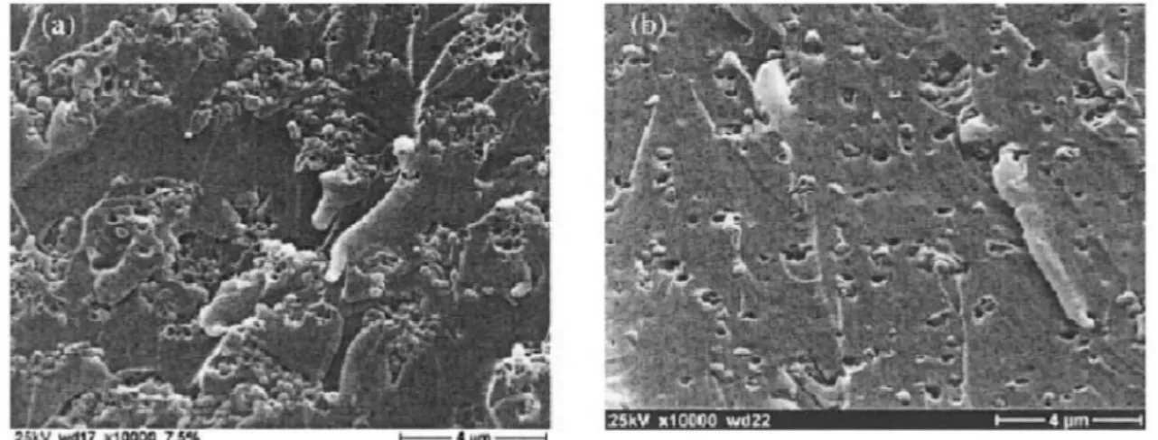
The level of dispersion can be examined with scanning electron microscopy (SEM) from the sample surface. The dispersion of titanium dioxide nanoparticles (Ø 300 nm) has been inspected from the epoxy fracture surface using SEM (Figure 2.5.). The nanoparticle agglomerates can be clearly seen in the Figure 2.5.a as compared to evenly distributed particles in the Figure 2.5.b. [1]

Figure 2.5. Fracture surface of epoxy resin with (a) undispersed (b) well dispersed

titanium dioxide nanoparticles [17]

2.3 Manufacturing

There are several different methods for incorporating the nanoparticles into the matrix: in situ polymerization, direct mixing and solvent mixing. In situ polymerization method incorporates the nanoparticles directly to the polymer chains by chemical methods. [17] It is suitable for raw polymer manufacturers. [19] Solvent mixing uses solvent, for example acetone or ethanol, to help breaking the agglomerates. Solvent must be removed before adding the hardener. [4] [26] Direct mixing is the most compatible method to use at the industrial level, because it allows production of nanocomposites with lower costs. [27] It is also environmentally safe without the solvents and contaminants that are used in solution method and in situ polymerization. [28] In direct mixing, the nanoparticles are added into the resin using, for example, high shear or sonication. High shear mixing can be done with rotating disc (Figure 2.6.), which breaks the agglomerates and distributes the particles evenly into the matrix polymer. Grinding by ceramic balls can also be used. [4] [17] Sonication is used only for small scale production, because the vibration energy works well only between small

(15)

7

distances. [29] In addition to processing methods described above, other techniques have been also developed including solid intercalation, covulcanization, and sol-gel method. Some of these are still being developed and not yet used widely. [19] High shear mixing is used in this work to manufacture epoxy nanocomposites and therefore it is elaborated further in the following chapter.

Figure 2.6. High shear mixing with a rotating disc [17]

High shear mixing is especially used for incorporating extremely fine filler particles into fluids, such as thermosetting resins. The high shear will first wet the particles surfaces by the fluid and then break down the particle agglomerates to smaller particles and distribute them evenly into the fluid. The shear is most effective at the tip of the dissolver disc, where the speed through the fluid is the highest. The circumference velocity can be calculated by the equation 1, where d is the dissolver disc diameter in meters and n is the rotating speed in rpm.

60 n d

v (1)

With a dissolver disc of Ø 50 mm and rotating speed of 4000 rpm (both used in this work) the circumference velocity is 10.5 m/s.

The mixing efficiency is affected by the geometry of the dispersion container, the diameter of the dissolver disc and its height in the container, the peripheral velocity and the rheological properties of the fluid. Usually the smaller distance between the disc and the container gives higher shear rates within the gap. During the high shear mixing the fluid should form a doughnut-like flow pattern (Figure 2.7.). It is a sign that the maximum mechanical power possible is being applied on the fluid and eventually all the fillers will reach the dissolver disc. The doughnut effect is affected by the viscosity of the fluid. With too low viscosity the fluid will splash and generate bubbles during mixing, and with too high viscosity the doughnut effect cannot be achieved. The

(16)

8

rotational speed used should be the highest possible to obtain the greatest peripheral velocity but not too high to be able to maintain the doughnut flow pattern. [30]

Figure 2.7. Doughnut effect [31]

In addition to the mixing method used, the dispersion of the fillers is also affected by the shape, size and specific surface area of the particles, total volume content of the fillers, mixing conditions [17], polarity of the matrix resin, surface treatment of the particles and the curing temperature of the resin. [4] Even if the dispersion during mixing has been successful, maintaining the stable dispersion until the materials has cured may become a problem due to the secondary agglomeration, which may occur after mixing. Elevated temperature may enhance the reagglomeration because the viscosity of the resin decreases in the very beginning of the curing process. Reagglomeration occurs more easily when the filler content is higher, because the distances between the particles are shorter. [23]

2.4

Matrix

materials

Polymers can be divided into thermoplastics and thermosets, according to their behaviour under temperature rise. Thermoplastics become softer when they are heated and harden back when they are cooled. This is a reversible process. When thermosets are heated, they become permanently hard. [32] This behaviour is based on the chemical reactions during curing. Thermoplastics have only physical changes where the polymer chains are entangling with each other. This makes it possible to repeat the softening and hardening cycles. [33] Both thermoplastics and thermosets can be used to make nanocomposites, and also elastomers are widely used. [18] [14]

Thermosets form a crosslinked network during curing, where covalent bonds are formed between the polymer chains. These bonds cannot be broken with re-heating. They resist the vibrational and rotational movements of the cured structure, which prevents the material to soften during temperature rise. [32]

When cured thermoset is heated above a certain temperature, they go through glass transition (Tg) temperature. Below Tg the material is glassy and hard, but after glass

(17)

9

transition temperature it changes into soft and flexible and loses its dimensional stability. Properties, such as tensile modulus, drop significantly. This is a reversible process, the polymer becomes glassy again after cooling back below Tg. [33] [34] When

the temperature is elevated further after Tg, the material will reach the degradation

temperature. [33]

Most thermosets need an extra component to be able to cure, which is often called hardener or curing agent. [35] The ratio of resin and hardener varies depending on the thermoset system. The right ratio is important, because small deviations may change the curing behaviour and mechanical properties of the final material. Mixing of the resin and hardener is done at room temperature or at elevated temperatures. The viscosity has to be low enough to achieve a homogeneous blend, which can be enhanced by heating the resin. However, the heating should be moderate in order to avoid the accelerated curing reaction, which can make the mixing and moulding difficult. [36] An example of the crosslinking is presented in Figure 2.8., where epoxy is cured with amine hardener.

Figure 2.8. Crosslinking network of epoxy resin with amine hardener [34]

When the thermoset is cured at elevated temperatures, the viscosity of the thermoset mixture (thermoset + hardener) decreases at the beginning of the temperature rise. As the curing is continued, molecular weight increases, which also causes the viscosity to increase. As the curing is continued further, the mixture starts to behave like a gel. [36] This phenomenon is called gelation. The gel point is the point in polymerization when the network structure first starts to occur. [33] As the structure develops, the network will stiffen and the glass transition temperature of the material will increase. [37] The gel point is also the time limit for the processing conditions when the moulding of the mixture is not possible anymore due to the extreme increase of the viscosity. This is why the shaping of the thermoset in the mould has to be done before the gel point. [36]

A common method to manufacture thermoset products is moulding. After the resin and hardener is mixed, the mixture is usually held under vacuum to remove the air bubbles that are usually formed during stirring. After that, the resin mixture can be

(18)

10

poured into the mould. The liquid resin fills the mould evenly and during curing it takes the shape of the mould. Curing is then performed for suitable time and temperature for the specific resin system. The sample can be removed from the mould after the curing is finished and the sample and the mould have cooled. [33]

The cured thermosets have many good properties, including solvent resistance, heat resistance, fatigue strength and excellent adhesion. [38] Thermosets have low viscosity in the beginning of processing, which enables less pressure and lower temperature during manufacturing than thermoplastics. [36] However, manufacturing of thermoplastic products takes generally less time than with thermosets, which is why they are better for high volume applications. [35] Thermosets are commonly used as the polymer matrix material in nanocomposites. [3] With thermoset resins the nanoparticles are used to reduce thermal shrinkage and brittleness, and to increase hardness, toughness and abrasion resistance. [1]

The most common thermoset resins are divided into polyester, vinyl ester and epoxy resins. Also phenolic and urethane resins are used. [38] Epoxy is a widely used thermoset resin in aircraft components and boat structures due to the good mechanical and adhesive properties and resistance to environmental degradation. Epoxy is also easy to process due to its low viscosity and relatively short curing time. [34] Epoxy is, however, more expensive than other thermoset resins like vinyl ester.

Epoxy has a long-chain structure that forms a three-dimensional network during curing. Epoxy groups form reactive sites in the chains that connect with the hardener. The epoxy group, circled in Figure 2.9., is a three-member ring, where two bonded carbon atoms are bound to one oxygen atom. Figure 2.9. shows also a typical structure of epoxy containing a monomer called diglycidyl ether of bisphenol A. The molecule contains two ring groups in the centre. They are able to absorb mechanical and thermal stresses, which offers good stiffness, toughness and heat resistance properties for the resin. [34]

Figure 2.9. Chemical structure of an epoxy group [34]

Curing agent for the resin is chosen by the curing conditions and the final application of the epoxy material. [33] Amines are widely used for curing because they have a good reactivity with epoxy and they are provided in wide variety. [39] Amines can be divided into aliphatics, cycloaliphatics and aromatics. Other curing agents include thiols and alcohols. Accelerators can also be used if the reaction is too slow for the application. [33]

Figure 2.10. shows curing of the epoxy with amine curing agents. In the first step the primary amine is added to the epoxy group. This is followed by the addition of the

(19)

11

secondary amine to add to another epoxy group. Hydroxyl groups accelerate the reaction by opening the epoxy ring. [39]

Figure 2.10. Curing steps of the epoxy with amine curing agent [39]

The curing treatment determines the properties, such as strength, stiffness and glass transition temperature, of the final material. Depending on the epoxy and the hardener, curing temperature can be somewhere between 5ºC and 150ºC. Usually the higher temperature gives better properties for the system. [34] [40]

Epoxy resins have a wide range of applications, including construction materials, automobile and aerospace applications, and as adhesives, coatings and electronic circuit board laminates. [41] The advantages of epoxy include excellent rigidity, high strength, low viscosity, low shrinkage during cure, chemical and thermal resistance, low creep and good adhesion to many substrates. [42] [1] Advantages compared to other thermosets include also low residual stresses in cured resin and minimum pressure that is needed during fabrication. Epoxy resin is available in many different viscosities, and the curing agents give many alternatives for different curing temperatures. [33] The disadvantages of epoxy are its brittleness in the cured state and poor resistance to crack growth. [1] Different nanoparticles can be used to improve the toughness of the epoxy, without degrading the properties of the epoxy resin. [42]

2.5 Nanoparticles

Inorganic nanoparticles can be divided into nanotubes (e.g. carbon nanotubes), layered silicates (e.g. montmorillonite), metals (e.g. Au, Ag) and metal oxides (e.g. Fe3O4,

TiO2). [43] There are also other carbon based nanomaterials like fullerenes [6], and also

nanofibers like cellulose whiskers [39]. The nanoparticles used in this work are presented in detail in the following chapters.

(20)

12

2.5.1 Layered silicates / Nanoclay / Montmorillonite

Layered silicates are clay minerals that can be either natural or synthetic. Natural clay called montmorillonite, belonging to the smectite family, is the most widely used clay as nanofiller. Synthetic clays like magadiite, mica, laponite and fluorohectorite are also widely used in nanocomposites. [39]

Montmorillonite clay was first found in Montmorillon, France in 1847. Nowadays it can be found in numerous places around the world. Montmorillonite is usually produced by weathering of eruptive rock material like volcanic ash or tuffs. Purification of other volcanic rock minerals like crystobalite and quartz is needed before usage. [39]

One layer of the montmorillonite clay is about 1 nm thick and the diameter can be from tens of nanometres to even microscale. The structure belongs to the class of 2:1 phyllosilicates. [44] They consist of two tetrahedral sheets of silica with an octahedral sheet of aluminium or magnesium hydroxide in the middle, as illustrated in the Figure 2.11. [39] Oxygen ions of the octahedral sheet are shared by the tetrahedral sheets. These 2:1 structures form stacks (about 8-10 nm thick [39]) of several layers that are held together by van der Waals forces. These forces are relatively weak, which enables an intercalation of small molecules (like polymer) between the layers. [44] Isomorphous substitution, where Si4+ can be replaced by Al3+ in the tetrahedral sheet or Al3+ by Mg2+ in the octahedral sheet, creates negative charges between the layers. [39] Those are counterbalanced by alkali or alkaline earth cations. [44] There are usually also water molecules present between the layers, because clay is very hydrophilic. [39] This is due to the hydration of exchangeable cations and the polar nature of the Si-O groups. [18] Clay particles can be modified to be more compatible with hydrophobic polymers. [39] The cations of the interlayer can also be exchanged with cationic surfactants, like alkylammonium or alkylphosphonium, to lower the surface energy between the layers and making it easier for the polymer molecules to intercalate into the galleries. [44]

(21)

13

The chemical formula of the montmorillonite is M_x(Al₄ _xMg_x)Si₈O₂₀(OH)₄. M is a monovalent cation, for example sodium ion, and x is the degree of isomorphic substitution (between 0.5 and 1.3). [45]

Mixing of the layered silicates is a complex process. In addition to the good dispersion of the particles, exfoliation of the layered platelets is also required to get the desired properties. According to the organizing of the clay particles in the matrix, the clay-nanocomposites can be divided into three types: phase separated microcomposite, intercalated nanocomposite and delaminated nanocomposite. These are presented in Figure 2.12. [44] In the phase separated microcomposite, the clay particles act as normal microscale fillers, because the polymer has not been intercalated between the clay layers. [39] [44] In the intercalated nanocomposite, the clay layers have moved slightly apart [40] and the polymer molecules have been moved between the layers. In the delaminated (also called exfoliated) nanocomposite, the clay layers have totally separated from each other [39] and dispersed as individual particles into the matrix. [22] This increases the number of reinforcing components [19] and the total surface area of the filler phase. [18] The entire surface of the clay layer is available for the polymer. [39] The platelets can be aligned or in random state. [22] The delaminated structure forms the “true” nanocomposite. [40], giving the maximum reinforcement for the composite. [18] However, the fully delaminated structure is very difficult to achieve. Conventional processing methods usually give a mixture of the three above mentioned structures. [22]

Figure 2.12. Different forms of clay-nanocomposite structures. [18]

Manufacturing of the clay-nanocomposites is usually done using in situ

polymerisation, melt intercalation or solution induced intercalation. In situ

(22)

14

galleries and dispersing the individual layers into the matrix by polymerisation. This method can produce well-exfoliated nanocomposites. It is suitable for raw polymer manufacturers to use in polymer synthetic processes. Melt intercalation combines the clay and polymer during melt processing. Even though it may not be as efficient as the

in situ method, melt processing has increased the commercial production of clay-nanocomposites. Solution induced intercalation uses solvents for swelling and dispersing the clay layers into the matrix. [19] Solvent method may not be the best option for commercial production since solvent has to be removed before adding the curing agent, and the solvents may be expensive. [4] [19]

Layered silicates are used as nanocomposite fillers to improve the mechanical properties, barrier properties, thermal resistance and fire resistance. [39] Barrier properties require the alignment of the clay plates, which creates a tortuous diffusion path. [22] Optical clarity occurs in exfoliated structure, because the nanometer-thick layer is much smaller than the wavelength of the visible light. [19] Nanoclays are also relatively cheap. [18] In epoxy, nanoclay is often used to improve thermal and mechanical properties in integrated circuit packaging and printed circuit boards, and also in coatings, automotive and aerospace industries. [46]

2.5.2 Carbon nanotubes (CNTs)

Carbon nanotubes are long chain-like structures that consist entirely of carbon. Other forms of pure carbon include fullerenes, and the more commonly known graphite, diamond and fullerenes. These different forms of carbon are presented in Figure 2.13. Graphite has a two-dimensional structure that consists of large planar sheets of aromatic rings with alternating single and double bonds (Figure 2.13.a). Diamond, on the other hand, has a three-dimensional structure that consists entirely of single carbon-carbon bonds in traditional 109° angles (Figure 2.13.b). [3] Properties of these two carbon allotropes are highly different from each other: diamond is transparent and one of the hardest materials known where graphite is black in colour and so soft that it can leave a mark on paper. [23] Fullerenes and carbon nanotubes are nanoscale structures. Fullerenes (Figure 2.13.c) consist of hollow spherical clusters where sixty carbon atoms are face-centered. Carbon nanotubes consist of graphite sheets rolled on a tube (Figure 2.13.d). [32] The ends of the tubes are usually closed with a structure of a half fullerene. [23] Carbon nanotubes and fullerenes can both be made as highly conductive or semiconductive. [32]

(23)

15

Figure 2.13. Allotropes of carbon: (a) graphite, (b) diamond, (c) fullerene, (d) carbon

nanotube [23]

Carbon nanotubes are a quite new discovery. Fullerenes were discovered first, by Robert F. Curl, Harold W. Kroto and R. E. Smalley in 1985. Their finding was later awarded by the Nobel Prize. [3] In 1991 Japanese scientist Sumio Iijima observed carbon nanotubes as a result of electric arc discharge technique. [23] The first discovered tubes were multi-walled, and single-walled tubes were found shortly after that. [47] Since then the carbon nanotubes have been under considerable research. [48]

The walls of the carbon nanotubes consist of the same structure as graphite sheets (Figure 2.14.a): hexagonally structured carbon atoms where each hexagon is a six-membered aromatic ring. [3] Carbon nanotubes can exist as single-walled or multi-walled tubes. A single-multi-walled tube, as in Figure 2.14.b, consists of one wall, while multi-walled tube, as in Figure 2.14.c, consists of several coaxial tubes. [40] Van der Waals forces between the tubes are keeping them together. [48]

Figure 2.14. (a) Graphite sheet, (b) single-walled carbon nanotube, and (c)

multi-walled carbon nanotube [49]

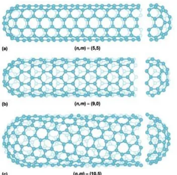
When the tube is thought of as rolled graphite sheet, the atomic arrangement of the hexagonal wall structure is defined by the rolling angle of the sheet. The structure has an effect on the transport properties, which defines the electrical and thermal conductivity of the tube. The atomic structure can be described by chirality, which is determined by the chiral vector Ch and chiral angle . The atomic arrangements are

(24)

16

categorized as ‘zig zag’, ‘armchair’ and ‘chiral’ (Figure 2.15.). They are described by the chiral vector C_h na₁ ma₂, where the integers n and m present the number of steps through the carbon bonds along the unit vectors a and ₁ a . The chiral angle ₂ determines the amount of ‘twist’ of the tube. In multi-walled carbon nanotubes each tube can have a different structure. [23] [40] [48]

Figure 2.15. Different carbon nanotube structures: (a) armchair, (b) zig zag, (c) chiral

[47]

Density of the carbon nanotubes is estimated to for the SWCNTs to be only 0.6 g/cm3 and for the MWCNTs between 1 and 2 g/cm3. [50] The diameter, being between 1-100 nm [51], depends on the number of aromatic rings that form the circumference of the tube. [3] The length of the tube can be up to millimetres. [51] This creates a very high aspect ratio [23], and the specific surface area of a single tube can be as high as 10-20 m2/g. [52] However, many processing methods reduce the tube length to about 100 nm for the final products. [3]

Carbon nanotubes have exceptional mechanical, thermal and electrical properties. Young’s modulus can be greater than 1 TPa [51], and strength can be even 100 times higher (about 150 GPa) than high strength steel. [53] Comparing single-walled and multi-walled tubes, the multi-walled tubes are stiffer than the single-wall tubes. [2] Carbon nanotubes are thermally stable up to 2800ºC in vacuum, and its thermal conductivity is higher than the one with diamond. Also, carrying capacity of electric current is 1000 times higher than in copper wires. [48] Therefore, CNT-composites are suitable for light-weight applications combined with high strength and electrical conductivity. [54] However, in order to have composite with such properties, nanotubes have to be evenly dispersed into the matrix. Due to their long and flexible structure combined with strong van der Waals forces between them, carbon nanotubes have an

(25)

17

extremely high tendency to agglomerate. [55] The commercial CNTs are usually supplied already as heavily entangled bundles [23], as in Figure 2.16., and their separation is very challenging. [55] Carbon nanotubes are used with very low filler contents.

Figure 2.16. Scanning electron microscope image of MWCNT bundles [56]

Single- and multi-walled carbon nanotubes can be produced with several different methods: arc-discharge, laser ablation, gas-phase catalytic growth from carbon monoxide, and chemical vapour deposition (CVD) from hydrocarbons. [48] Arc-discharge method is based on a direct current going through two high-purity graphite electrodes under helium atmosphere. High volumes of single-walled and multi-walled tubes can be produced. [40] Laser ablation method was earlier used for the initial synthesis of fullerenes, but it is now developed to produce single-walled carbon nanotubes. Laser ablation is based on laser associated vaporization of graphite and its condensation on a water-cooled target. Both arc-discharge and laser-ablation methods are limited by the low volume production and the necessary of purification from the undesired by-products. Chemical vapour deposition (CVD) is a gas-phase technique where the decomposition of carbon-containing gas forms carbon nanotubes. A direct current between two electrodes produces plasma where carbon is vaporized from the anode and reorganized at the cathode. This forms a cylindrical deposit of un-aligned graphite planes, where multi-walled tubes are forming. [17] This is a continuous process that enables high yield of the tubes. CVD is able to control the diameter and length of the tubes, and purification is less needed. [48]

Carbon nanotubes are used with polymers to increase mechanical, thermal and electrical properties. [57] Carbon nanotubes have a great potential for reinforcement, because they are the stiffest fiber known. They could be used to replace glass and carbon fibers in polymer composites [58], but the challenges with the production techniques and the raw material price has to be overcome before they can be used to produce cost-effective composites. [48] Potential applications for CNT-filled nanocomposites are coatings, sensors, probes, energy storage devices, field emission displays, lightweight vehicles, aircrafts, civil constructions, sports equipments, marine, and military hardware. [57]

(26)

18 2.5.3 Silicon dioxide (SiO2)

Silica (SiO2), or silicon dioxide, belongs to the silicate materials, which are primarily

composed of silicon and oxygen. Silicate materials include the bulk of soils, rocks, clays and sand. Structure of silicate materials consist of SiO₄4 -tetrahedrons, with one silicon atom in the middle and four oxygen atoms at the corners. Different silicate materials consist of different arrangements of the tetrahedron. Silica is the most simple silicate structure. It is a three-dimensional network, where every corner oxygen atom of each SiO₄4 -tetrahedron is shared by the neighbouring tetrahedron (Figure 2.17.). Bonds between the silicon and oxygen atoms are strong, which results in high melting temperature (1710°C). [32]

Figure 2.17. Chemical structure of silicon dioxide (SiO2) [59]

Silica can exist in crystalline or amorphous form. [60] The primary forms of crystalline silica are quartz, trydimite and cristobalite. [32] Natural quartz constitutes 12,5% of the Earth’s crust. [21] Amorphous silica and the part of the crystalline silica forms can be divided into natural and synthetic products. [60] Generally the different forms of silica include fused quartz, crystal, fumed and colloidal silica, silica gel and aerogel. Applications of silica include electronics, ceramics, polymer industry and concretes in construction industry. [61]

Nanosized silica has a density of 1.09-1.3 g/cm3 and diameter of the spherical particle can be only 4 nanometers. [21] Nano-SiO2 can be produced with several

methods, including sol-gel process, vapour-phase and thermal decomposition technique. [61] Commercial nano-SiO2 powder is usually fine and white amorphous powder

produced by a fuming method. It is a high-temperature vapour process where SiCl4 is

hydrolyzed in an oxygen-hydrogen flame according to the reaction

4HCl

SiO

O

2H

(27)

19

Silica has a hydrophilic nature because of the silanol and siloxane groups that are formed on the silica surface. [43] Mixing of the hydrophilic silica with hydrophobic epoxy resin can be challenging due to their different polarities. [62] Furthermore, the silanol groups (Si-OH) on the adjacent particles (Figure 2.18.) form hydrogen bonds that hold the individual silica particles together creating agglomerates, which can be difficult to break. [43]

Figure 2.18. Hydrogen bonding among the silanol groups between silica particles [43]

Nano-SiO2 is widely used in different kind of industries including cosmetics, drugs,

printer toners, varnishes and biotechnological applications such as cancer therapy and drug delivery. [60] Technological applications include thixotropic agents, thermal insulators and composite fillers. [61] Nano-SiO2 has been used with thermoset resins to

increase the fracture toughness, impact strength, tensile modulus, durability and abrasion resistance, and to improve dielectric properties, heat distortion and chemical resistance. [17]

(28)

20

3 EXPERIMENTAL

3.1 Materials used in this study

3.1.1 Resin

Epoxy resin and curing agent used in this study were PRIMETM 20LV and PRIMETM Slow hardener, respectively. PRIMETM 20LV is a bisphenol A based epoxy resin and PRIMETM Slow hardener is an amine based hardener. Slow hardener gives a working time of one hour at room temperature for pure resin. The mixing ratio of the resin and the hardener was 100:26 by weight and the curing was done in oven at 65°C for 7 hours.

Table 3.1. Properties of the epoxy resin and hardener [63]

PRIMETM 20LV

resin

PRIMETM Slow

hardener

Supplier Gurit Gurit

Density (g/cm3) 1.123 0.936

Mixing ratio (by weight) 100 26

Viscosity at 20°C (cP) 1010-1070 22-24

Viscosity at 25°C (cP) 600-640 15-17

Viscosity at 30°C (cP) 390-410 12-14

3.1.2 Nanofillers

Three different nanofillers were tested in this study: nano-SiO2 (nanosilica), nanoclay

and carbon nanotubes (Table 3.2. and Figure 3.1.). Multi-walled carbon nanotubes and nano-SiO2 were both purchased from Sigma-Aldrich while nanoclay (trade name

Cloisite 11) was from Rockwood Clay Additives. Carbon nanotubes have outer diameter of 6-9 nm, length of 5 µm and the number of walls between 3 and 6 and they are produced by catalytic chemical vapour deposition (CVD) method. [64] Spherical nano-SiO2 particles have diameter of 12 nm and they do not have any surface treatment

according to the manufacturer. [65] Cloisite 11 is based on natural bentonite (consists mostly of montmorillonite) and the surface treatment is based on a quaternary ammonium salt. The diameter of the clay platelets is under 40 µm. [66] The prepared samples for tensile tests are presented in Figure 3.2. Filler contents by weight and volume are presented in Tables 3.3 and 3.4.

(29)

21

Table 3.2. Commercial nanofillers used in the work

Trade name Supplier Density [g/cm3]

Multi-walled carbon nanotubes Sigma-Aldrich 1.7 *

Silica nanopowder Sigma-Aldrich 1.1 **

Cloisite 11 Rockwood Clay Additives 1.6 *** * [67], ** [21], *** [68]

Figure 3.1. Pure powder of nanoparticles: (a) nano-SiO2, (b) nanoclay, (c) MWCNT

Figure 3.2. Tensile test samples and sample concentrations

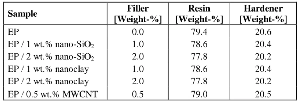
Table 3.3. Filler contents in manufactured samples (by weight)

Sample Filler [Weight-%] Resin [Weight-%] Hardener [Weight-%] EP 0.0 79.4 20.6 EP / 1 wt.% nano-SiO2 1.0 78.6 20.4 EP / 2 wt.% nano-SiO2 2.0 77.8 20.2 EP / 1 wt.% nanoclay 1.0 78.6 20.4 EP / 2 wt.% nanoclay 2.0 77.8 20.2 EP / 0.5 wt.% MWCNT 0.5 79.0 20.5 ID Sample 1 EP 2 EP / 1 wt.% nano-SiO2 3 EP / 2 wt.% nano-SiO2 4 EP / 1 wt.% nanoclay 5 EP / 2 wt.% nanoclay 6 EP / 0.5 wt.% MWCNT

(a)

(b)

(c)

(30)

22

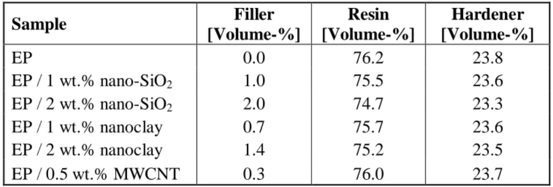
Table 3.4. Filler contents in manufactured samples (by volume)

Sample Filler [Volume-%] Resin [Volume-%] Hardener [Volume-%] EP 0.0 76.2 23.8 EP / 1 wt.% nano-SiO2 1.0 75.5 23.6 EP / 2 wt.% nano-SiO2 2.0 74.7 23.3 EP / 1 wt.% nanoclay 0.7 75.7 23.6 EP / 2 wt.% nanoclay 1.4 75.2 23.5 EP / 0.5 wt.% MWCNT 0.3 76.0 23.7

(31)

23

3.2 Sample preparation

Before mixing, the nanofillers were dried overnight in an oven at 80ºC to remove the absorbed moisture from the structure. Manufacturing process was started by pre-heating the resin in an oven at 40°C to reduce the viscosity. The mixing chamber was also heated with a water circulation to 40°C. Mixing of the hardener was done at room temperature, but the resin was usually still a little warm, about 30°C. Mixing was performed with high shear mixer Dispermat CA-40 (Figure 3.3.a) and a cogged mixing head with a diameter of 50 mm (Figure 3.3.b). Mixing of the nanofillers was done under vacuum (0.7-0.75 bar) for 60 minutes with a rotating speed of 4000 rpm. During mixing, the temperature of the mixture was raised to 45-56°C (MWCNT-filled mixtures increased more than others) due to friction. After the nanofiller mixing, the hardener was mixed to the nanofiller doped resin under vacuum (0.7-0.75 bar) with a rotating speed of 500 rpm for 2 minutes. The maximum amount of material that can be mixed at a time under vacuum is 200 ml.

Figure 3.3. (a) Dispermat CA-40 high shear mixer, (b) mixing head and (c) vacuum

chamber

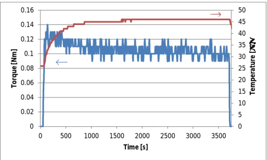
Temperature rise during the nanofiller mixing can be seen from the mixing data collected during mixing of the sample EP/1 wt.% of nano-SiO2 in Figure 3.4. As the

temperature rises, the torque decreases, which is indicative of viscosity decrease due to the higher temperature.

(32)

24

Figure 3.4. Mixing data of the sample EP/1 wt.% nano-SiO2

Air bubbles were formed into the resin during the high shear mixing of nanofillers and they were removed before the addition of hardener in a separate vacuum chamber (0.7-0.8 bar), presented in Figure 3.3.c. During vacuuming the mixture cooled down, which made it necessary to heat the resin in an oven (40ºC) between the vacuum cycles to lower the viscosity. Lower viscosity of the nanofilled resin made the removal of the bubbles more efficient. Vacuum cycles were repeated for necessary times, depending on the amount of air bubbles in the structure.

Mixing of the hardener was done at room temperature to avoid a catalytic reaction caused by the nanofillers and their surface treatment. This catalytic effect decreased the working time of epoxy significantly and it was noticed especially when using nanoclay. This may indicate that the nanoclay was not compatible with the epoxy resin. The hardener was mixed with lower speed and shorter time to reduce the formation of new bubbles. If a notable amount of bubbles formed, the mixture was held under vacuum for a maximum of 30 minutes after adding the hardener. The manufacturing procedure is presented also in Figure 3.5.

0 5 10 15 20 25 30 35 40 45 50 0 0.02 0.04 0.06 0.08 0.1 0.12 0.14 0.16 0 500 1000 1500 2000 2500 3000 3500 Te m pe ra tu re [ ° C] To rq ue [N m ] Time [s]

(33)

25

Figure 3.5. The thermoset nanocomposite sample preparation process

Metal frames (Figure 3.6.) were used for moulding the samples. They were placed on top of steel plate (thickness 10 mm), which was covered with a PTFE sheet. In addition, the frames were treated with a mould release agent (Chemlease 75) before moulding. Bone-shaped frames were used to manufacture tensile test samples (type 1A test bar according to standard SFS-EN ISO 527-2). Furthermore, fracture toughness samples were cut from the square samples (size 8 mm x 35 mm). Six tensile test samples (thickness 4 mm) and 2 square samples (thickness 4 mm) were manufactured from each material. The filled moulds were kept at room temperature for two hours to allow the air bubbles to come on the surface. Curing was done at 65°C for seven hours.

(34)

26

3.3 Characterization

3.3.1 Viscosity

Viscosity measurements were used to examine the flow properties of the nanofilled resins. Viscosity can be used to analyse the dispersion of the nanoparticles and the interaction between resin and the fillers. [1]

Viscosity measurements were done with Anton Paar’s rotational rheometer Physica MCR 301 (Figure 3.7.a). Plate-plate configuration (Figure 3.7.b) was used with a 1 mm gap. Viscosity was measured as a function of temperature between 23°C and 65°C with a shear-rate of 10 1/s, and as a function of shear rate between 0.1 and 100 1/s at room temperature (Table 3.5.). Oscillating measurement was also done for samples with nano-SiO2 contents of 2 and 4 wt.%. Different gap distances were experimented with 4

weight-% of nano-SiO2. All the measurements were performed to the nanofilled resin

without the hardener, so the filler amount was somewhat higher than in the final samples.

Figure 3.7. (a) Physica MCR 301 rotational rheometer, (b) Plate-plate configuration

Table 3.5. Viscosity measurement parameters

Mode Function Temperature Shear rate Configuration

Shear Temperature 23°C - 65°C 10 1/s Plate-plate (1mm gap) Shear Shear rate Room temp. 0 - 100 1/s Plate-plate (1mm gap) Oscillating Temperature 23°C - 65°C 10 1/s Plate-plate (1mm gap)

(35)

27 3.3.2 Tensile test

Tensile test was performed to the samples in order to analyze their mechanical properties. Tensile test gives information about the tensile strength and modulus of the samples. The force that is needed to break the sample and the elongation until the breaking point are measured during the test. Modulus can be calculated from the data of the stress-strain curve. [69]

Tensile strength is the maximum tensile stress that is recorded during tension. [70] It is very dependent on the interactions between the matrix and the fillers. [18] Tensile stress can be calculated with the Equation 3:

A F

(3)

where F is the force in Newtons (N), and A is the cross-sectional area of the sample in square millimetres (mm2). [71] Modulus describes the material’s resistance to deformation. [18] Young’s modulus E is calculated from the ratio of the stress difference between and and the strain difference between and (Equation 4). The strain difference between = 0.0005 and = 0.0025 was used in the measurements, according to standard SFS-EN ISO 527-1. [71]

1 2

E (4)

An extensometer (Figure 3.8.b) was used to measure the elongation. Extensometer measures the elongation from the narrow part of the sample, because the bone-shaped tensile test sample does not elongate uniformly. [72]

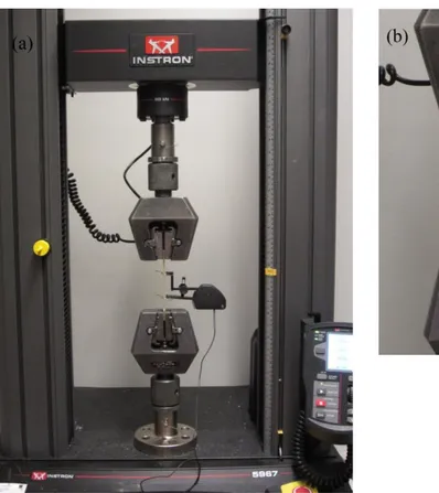
Tensile tests were performed with Instron 5967 tensile test machine according to standards SFS-EN ISO 527-1 and SFS-EN ISO 527-2 using a load cell of 30 kN. The tensile test arrangement is presented in Figure 3.8.a. Thickness, length and width of the narrow portion in the tensile test samples (presented in Figure 3.2.) were 4mm, 150mm and 10mm, respectively. The draw rate of the test was 2 mm/min, gauge length in extensometer 50 mm and the frequency 0.417 1/s. Prior testing, all samples were stored in a humidity room for a few days.

(36)

28

Figure 3.8. Tensile test (a) The arrangement (b) The extensometer

3.3.3 Fracture toughness

Fracture toughness analysis was used to measure the ability of a sample with an existing crack to resist a fracture. Fracture toughness sample is a notched rectangular where a natural crack is cut by a razor on the notch. Fracture toughness analysis can be used to design materials for dynamic applications. It is a very useful test method because it is almost impossible to make a material without any cracks or defects. [33] The theory behind the improved fracture toughness of nanocomposites is the creation of torturous path due to the well dispersed nanoparticles. In that case, the crack propagates along the nanoparticles producing a larger fracture surface area. [73]

Fracture toughness test was determined by standard ASTM D5045-99 with a single-edge-notch bending (SENB) configuration. The critical stress intensity factor KIc, that

can be used to analyze the resistance to fracture, is determined with the equation 5:

f(x) BW

P

K_Ic Q_1/2 (5)

Where PQ is the critical load for crack propagation, B is the thickness and W is the

(37)

29 3/2 2 x) 2x)(1 (1 ) 2.7x 3.93x x)(2.15 x(1 1.99 x 6 f(x) (6)

where a is the crack length (machined notch plus razor crack) and x = a/W. [33] [74] Fracture toughness sample (Figure 3.9.) is a notched rectangular, where a natural crack is cut on the notch by a razor. Fracture toughness sample dimensions were 8 mm x 4 mm x 35 mm and they were cut from the square samples with a disc cutter (using water). The 4 mm deep notch was cut with a circular saw (dry) and the natural crack (length about 0.1 mm) was mad by a sharp knife at the tip of the notch. Six samples from each material were tested and the samples were stored in a humidity room for a few days before testing.

Figure 3.9. The fracture toughness sample

Tests were performed with Instron 5967 tensile test machine using a rate of 3mm/min and a load cell of 30 kN. A special bending fixture was used for the tests (Figure 3.10.b), where the upper tensile jaw moved freely upon the fixture (Figure 3.10.a). The force created by the weight of the upper jaw, 9N, was added on the results since the weight was already on the sample before the test started. The fracture toughness sample was placed on the fixture with the notch pointed down like it is shown in Figure 3.9.

Figure 3.10. Fracture toughness: (a) Test arrangement, (b) Test fixture

Upper jaw

(38)

30

3.3.4 Differential scanning calorimetry (DSC)

Differential scanning calorimetry was used to determine the degree of cure and the glass transition temperature of the samples. [72] DSC is based on a temperature difference between the sample (weight generally between 5-10 mg) and the reference material during heating or cooling. [75] [72] An electric signal, given by the temperature difference, is converted to a heat-flow signal which is plotted against temperature. [75] Two heating cycles are usually performed for polymers, because the first one is strongly affected by the thermal history of the sample. [72] If the sample is not fully cured, some residual curing may occur during the first heating, which can be seen as an exothermic peak on the results. During the second heating, the test produces only glass transition peak. [76] The higher is the glass transition temperature, the higher is the degree of cure. [77] An increase in Tg with fillers is considered to result from strong interaction

between the filler and the matrix. Reduction in Tg is an indication of reduction in

crosslink density. [78] The mid-point temperature of the Tg curve is the most commonly

used definition for the glass transition (presented in Figure 3.11.). T1 and T2 are the onset and endset temperatures respectively, Tb represents the very beginning of the change in heat flow and the Te the very end of the detection of the glass transition event. [79] The sample does not necessarily have to be fully cured, thermoset samples can also be analyzed as uncured or partially cured. Heat development can be then monitored during curing. [33]

Figure 3.11. Determination of the Tg [79]

The DSC analysis was performed with Netzsch DSC 204F1 instrument, presented in Figure 3.12.a. The test sample and the reference can be seen in the middle of the Figure 3.12.b in the chamber. The samples were heated two times from 20°C to 270°C at a heating rate of 20°C/min under nitrogen atmosphere. Generally only one measurement was done for each sample, but pure epoxy and the sample EP/0.5 wt.% of MWCNT was tested twice.

(39)

31

Figure 3.12. (a)DSC instrument, (b) Sample and the reference inside the test chamber

3.3.5 Dynamic mechanical analysis (DMA)

Dynamic mechanical analysis was used to examine the effect of nanofillers on the viscoelastic properties of the resin. [1] Under external loading, the viscoelastic materials have a behaviour that varies between elastic and viscous. Totally viscous system converts all work as heat and cannot be recovered after the force is released. Totally elastic system is able to store all work as potential energy. [24] [3] DMA is able to give information about both of these properties as a function of temperature. [72]

DMA applies a small deformation on the sample and examines the stiffness of the sample. [80] Storage modulus (E’) gives information on the elastic properties, and loss modulus (E’’) on the viscous properties of the sample. [1] Tan measures the energy dissipation of the material and it is the ratio between the loss and storage modulus. [80] The higher the tan value is, the better the damping performance of the material. [15] Glass transition temperature can also be determined by the results, but the determination varies with industry. Most commonly the Tg is defined by the onset of the E’ drop, the

peak of the tan delta or the peak of the E’ curve. [80] In this work the Tg was

determined by the peak of the tan delta curve.

Dynamic mechanical analysis measurements were performed with Perkin Elmer Pyris Diamond DMA (Figure 3.13.) with three-point bending mode and frequency of 1 Hz. The samples were sawed from the square samples to the size of 3 mm x 4 mm x 40 mm. The temperature range used was 20-340°C with a heating rate of 2°C/min under nitrogen (inert) atmosphere. Only one measurement was done for each sample.

(40)

32

Figure 3.13. DMA instrument

3.3.6 Thermogravimetric analysis (TGA)

Thermogravimetric analysis was used to study the thermal stability of the samples. During TGA test, the mass of the sample is continuously recorded either as a function of time in isothermal mode or as a function of temperature in dynamic mode (the most widely used method [72]). [75] Test atmosphere can be either inert or oxidizing. [72] The mass loss of the sample gives information about the thermal decomposition of the samples and the volatile contents of the material components. [75]

Thermogravimetric analysis was performed with PerkinElmer STA 6000 (Figure 3.14.). Samples were heated from 25°C to 995°C with a heating rate of 10°C/min under nitrogen (inert) atmosphere. Only one measurement was done for each sample. Pure epoxy and the sample EP/0.5 wt.% of MWCNT was tested also under oxygen atmosphere.

(41)

33

Figure 3.14. TGA instrument

3.3.7 Scanning electron microscopy (SEM)

Scanning electron microscope can be used to inspect the fracture structure of the samples, analyse the dispersion of the nanoparticles and study the arrangement, distribution and geometrical features of nanofillers. [23] Scanning electron microscope produces topographical images with high resolution [33] and it is based on a focused beam of high-energy electrons that is focused on the sample surface. The beam produces signals from the sample that are based on the interactions between the sample surface and the electrons. [81] This requires that the sample has a moderate electrical conductivity [23] to prevent charging. Therefore the sample surface is coated with gold or carbon. [33] The primary electron beam that sweeps over the sample generates secondary electrons, backscattered electrons, Auger electrons and x-rays. Secondary electrons produce the topographical images of the samples. Auger electrons and x-rays can be used to analyse the spectroscopic or chemical composition of the sample. [23]

Philips XL-30 scanning electron microscope (Figure 3.15.) was used for the examination of the fracture surfaces of the tensile test samples using an acceleration voltage of 15 kV. Before the examination, the specimens were coated with gold.

(42)

34

Figure 3.15. Scanning electron microscope Philips XL-30

3.3.8 Field emission scanning electron microsopy (FESEM)

The nanoparticle dispersion was characterized also with field emission scanning electron microscope (FESEM). The advantage compared to conventional SEM is the high resolution with low accelerating voltages that enables to analyze nanostructures and other delicate materials like biological samples. [82]

FESEM Zeiss ULTRAplus (Figure 3.16.) was used to perform the FESEM analysis using an acceleration voltage of 5 kV. The examined surface was cut by liquid nitrogen from the tensile test samples and covered with carbon to make the sample conductive.

Figure 3.16. Zeiss ULTRAplus field emission scanning electron microscopy [83]

3.3.9 Electrical conductivity

Polymeric materials are generally good insulators with the surface resistivity value ranging from 1014 to 1018 ohm. Conductivity can be increased (resistivity decreased)

(43)

35

with the compounding with carbon based fillers. [84] Resistivity of carbon nanotubes is 5-50 µ cm. [52] With polymers, resistivity is often measured from the surface, while metals are usually measured through the volume due to their high conductivity. [84] The measurements are based mostly on the standard ASTM D 257-99: Standard Test Method for DC Resistance or Conductance of Insulating Materials.

In this study, electrical conductivity was measured only with the sample EP/0.5 wt.% of MWCNT (sample size 10 cm x 10 cm, thickness 4 mm). Prior to testing, the samples surface was cleaned with acetone and paper towel. Measurement was done attaching two electrodes to the sample surface with 500 volts between them. Dimensions of the electrode are presented in Figure 3.17.

D1 = 3.00 cm D2 = 5.70 cm D3 = 6.35 cm g = D2 - D1 = 1.35 cm D0 = D1 + g = 4.35 cm P = ð * D0 = 13.67 cm

Figure 3.17. Electrode dimensions

Surface resistance is measured using the equation Rs= U/I (where Rs is surface

resistance, U is voltage and I is current). Surface resistivity is measured using the surface resistance and the equation Ps=(P·Rs)/g. The ratio P/g using the electrodes

described above is 10.123 (= 13.67mm/1.35mm), so the surface resistivity can be calculated by multiplying the surface resistance with this constant.

Volume resistance can be calculated with the equation Rv= U/I. Volume resistivity

·cm), on the other hand, is calculated with the equation Pv = (A·Rv)/t, where t is the

sample thickness and A is calculated using the equation 7. [85]

2 2 cm 14.86 4 g) (D1 A (7)

(44)

36

4 RESULTS

4.1 Viscosity

4.1.1 Viscosity observations during processing

Considerable differences in the viscosities of the nanofilled epoxy resin samples were observed during manufacturing. The high viscosity of the samples EP/2 wt.% nano-SiO2

and EP/2 wt.% nanoclay made the removal of the air bubbles after mixing challenging. Both samples had to be vacuumed and heated several times so that the casting of the samples was done on a following day after the first mixing. With the sample EP/2 wt.% nanoclay, several vacuuming and heating cycles enhanced the air bubble removal resulting samples, which were free of visible air bubbles. For sample EP/2 wt.% SiO2,

similar amount of air bubbles was left on the resin when casting the samples after only a few times of vacuuming and heating than with continuing the vacuuming process until the next day. The vi