The generalised Cornu spiral and its application
to span generation
J.M. Alia, R.M. Tookeyb, J.V. Ballb, A.A. Ballb;∗
a
School of Mathematical Sciences, The University of Science Malaysia, 11800 Minden, Penang, Malaysia
bSchool of Manufacturing and Mechanical Engineering, The University of Birmingham, Edgbaston, West Midlands,
B152TT, United Kingdom
Received 12 January 1998; received in revised form 23 June 1998
Abstract
A Cornu spiral is a plane curve having a linear curvature prole. This paper considers plane curves having rational linear curvature proles. These curves are dened to be generalised Cornu spirals (GCS) and are quality curves in the sense that they are continuous and smooth, can contain one inection at most, and have a bounded and monotonic curvature prole. In addition, the GCS has an extra degree of freedom over the Cornu spiral that is available for shape control. Starting from the intrinsic equation of the GCS, the technique of curve synthesis is used to design a quality curve that can be applied to a wide range of span generation problems. c 1999 Elsevier Science B.V. All rights reserved. Keywords:Generalised Cornu spiral; Curve synthesis; Span generation
1. Introduction
Over the last 25 years, there has been an increasing interest in the synthesis of curves and surfaces for Computer-Aided Design. This has stemmed from engineers wanting to design surfaces with guaranteed geometric properties, rather than the more customary, and time-consuming, practice of constructing a surface and then interrogating and rening it until it has the necessary characteristics [9]. In other words, engineers want to ensure quality by design.
Much of the current research was initiated by Nutbourne et al. in 1972 [10]. They developed a technique for constructing plane curves by integrating their curvature proles. The work is based upon the Fundamental Theorem for Space Curves which states that if two single-valued continuous functions (s) and (s), s ¿0, are given, then there exists a unique space curve r(s), determined up to a rigid-body motion, for which s is the arc-length, the curvature and the torsion [14]. Setting
∗Corresponding author. Tel: 121 414 4150; fax: 121 414 3515.
(s) = 0, the theorem can be applied to plane curves. Various curvature proles were investigated in [10] and applied to several span generation problems.
There has been particular interest in linear curvature segments which correspond to arcs of Cornu spirals. Pal and Nutbourne [12] proved that at least two linear curvature segments are required to interpolate end points, tangents and curvatures, and discussed quality issues for solutions with two and three segments. Schechter [13] presented an interactive approach requiring up to ve segments for a satisfactory span synthesis. More recently Meek and Walton [7] have presented an alternative solution with conditions for existence and uniqueness.
This paper presents a practical engineering solution to the span generation problem, using a single arc from a generalised Cornu spiral (GCS) [2]. The GCS has a rational linear curvature prole and, by denition, is more versatile than the Cornu spiral in shape description. It is a quality curve in the sense that it has a monotonic curvature prole [3, 6]. However it is not in general possible for a GCS (nor any curve with a monotonic curvature prole) to interpolate specied end points, tangents and curvatures. For example if the two end curvatures are equal then the blend curve must be a circular arc which is unlikely to be geometrically consistent with the endpoints and tangents. In engineering applications it is often preferable to resolve such inconsistencies by introducing small discontinuities in curvature [4] rather than comprising the monotonic variation of curvature. Consequently, the GCS construction in this paper matches the end points and tangents but only approximates the end curvatures.
2. Intrinsic equation of a curve
Without any loss of generality, this paper considers arc-length s parametrised curves lying in the
xy plane, i.e., r(s) = [x(s) y(s)], 06s6S, where S corresponds to the total arc-length. For plane curves, it is straightforward to dene the unit tangent vector t(s), the unit normal vector n(s) and the (signed) curvature (s) directly from r(s) using
t(s) =
dx(s)
ds
dy(s) ds
; n(s) =
−dy(s)
ds
dx(s) ds
and
(s) =dx(s) ds
d2y(s)
ds2 −
dy(s) ds
d2x(s)
ds2 ;
where a positive (s) corresponds to a counter clockwise rotation of the tangent.
Conversely, for a given curvature prole (s), 06s6S, it is possible by successive integrations to determine t(s) and r(s) up to a rigid-body motion [14]. This process is referred to as curve synthesis.
Let (s), 06s6S, be dened as the (signed) angle (in radians) from the positive x axis to t(s) such that
t(s) = [cos(s) sin(s)];
where
(s) =(0) +
Z s
0
Integrating again gives
Eq. (2) thus provides the equation of the curve from its curvature prole. The integrals contained in the above equation, called Fresnel integrals, cannot be integrated in general and numerical techniques are required to generate points on the curve (cf. [10, 1]).
3. Generalised Cornu spiral
A GCS is dened to be a curve having a rational linear curvature prole [2]. In its normalised form, (s), 06s6S, is given by
Dierentiating Eq. (3) with respect to s gives
d(s) dierentiable (smooth) since d(s)=ds is continuous.
As noted at the end of the previous section, there is no explicit curve equation for the GCS unless the curvature prole is linear [10], i.e., r= 0. Suppose r6= 0, then Eq. (3) can be integrated to give
(s) =(0) + (pr−Sq)
and Eq. (2) has to be integrated numerically. The four available degrees of freedom, namely p, q, r and S, together with the predictable nature of the inection, should provide sucient exibility for a wide range of shapes. In the next section, the span generation problem is framed with respect to the GCS.
4. Span generation
The GCS has proven shape qualities and is therefore an ideal candidate as a blend or transition curve [6]. This section formulates the span generation problem with respect to the GCS.
Consider two distinct points r0 and r1 with specied unit tangent vectors t0 and t1 and specied curvatures 0 and1. Suppose0 and1 are associated witht0 andt1 respectively. The ideal solution
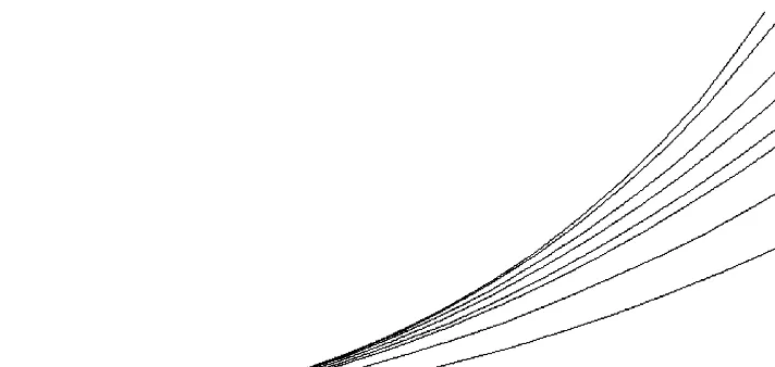
Fig. 1. Family of GCSs with various values of the shape factorr.
ends. Note that, as yet, the length of the span S has not been specied. The problem is approached from an intrinsic perspective, hence the curvature constraints are rst considered, followed by the tangent and then the position constraints.
For the GCS to match the end curvatures, (s) must satisfy (0) =0 and (S) =1. Substituting
into Eq. (3) gives
(s) =(S−s)0+ (1 +r)s1
S+rs (5)
which eliminates p andq and leaves only r and S as free parameters. Sincer controls the curvature prole and hence the shape of the GCS, it is referred to as the shape-factor.
Fig. 1 shows a family of GCSs with 0= 0:010, 1= 0:005, S= 100 and r=−0:9999;−0:9;−0:5;
0:0;1:0;2:0;10:0 and 10 000. The most highly curved segment corresponds to r=−0:9999 and the attest to r= 10 000. The gure demonstrates the extra versatility of shape control with a GCS compared to the Cornu spiral (r= 0:0) whose ends are marked with small circles.
Integrating Eq. (5) (cf. Eq. (4)) gives
(s) =(0) +Sm(s)0+ (s−Sm(s))1; (6)
where
m(s) =S(1 +r)ln (1 + (rs=S))−rs
Sr2 (7)
is a continuous function of s provided r6= 0. Expanding ln (1 +rs=S) as a Maclaurin series and then substituting into the above expression gives
m(s) = s S
1− s
2S
−rs
2
S2 1
2− s 3S
+r
2s3
S3 1
3− s 4S
+o(r2)
Provided 06=1, then Eqs. (1) and (6) can be equated to give an alternative expression for m(s), and m(r; s). Partial dierentiation of Eq. (5) with respect to r gives
@(r; s) @r = −
s(S−s)(0−1)
(S+rs)2 ;
which is also a continuous function of r and s, hence Leibniz’s rule [15] can be applied to give
@m(r; s)
This expression constrains the arc-length S. When 0=1,
S= (1−0)=1;
since 0¡ m(S)¡1, and the GCS matching the end tangents and curvatures has the unique shape-factor r satisfying
Integrating Eq. (6) (cf. Eq. (2)) gives
and
y1=y0+ Z S
0
sin(0+Sm(t)0+ (t−Sm(t))1) dt: (13)
Eqs. (12) and (13) can both be rewritten as nonlinear equations in r, using Eqs. (7) and (10). They are unlikely to have a common solution, since x1 and y1 can be varied independently. This
conrms that a single GCS cannot in general match the specied end points, tangents and curvatures. However, a practical solution is presented in the next section in which the end curvatures are only approximated. In curvature approximation it is more meaningful to consider percentage errors rather than absolute errors. As a rule of thumb, a 5% discrepancy in curvature is just visible irrespective of the curvature value. Consequently, the general aim of the GCS construction is to minimise the percentage discrepancies in the end curvatures, and the expectation is that for well-conditioned data the discrepancies will be small.
0 and 1 were introduced as the specied end curvatures but throughout this section they have
also denoted the end curvatures of the GCS. Now that GCSs are to be constructed which do not necessarily match the specied end curvatures, there is a need to clarify the notation. For consistency with all the numbered equations in this section, 0 and 1 are dened as the end curvatures of the
GCS. Indeed, Eq. (5) can be taken as the denition of a GCS; with 0, 1, r(¿−1) and S(¿ 0)
being the free parameters of the arc. Consequently, in the next section, the values of 0 and 1 are
initially assigned to match the specied end curvatures but are subsequently adjusted by a minimal amount so that the GCS matches the end points and tangents.
5. A practical solution to span generation
Without any loss of generality, the problem is approached via the special case where r0 is the origin and t0 is the unit vector in the direction of the positive x axis, i.e., x0=y0=0= 0. It is noted that the span data can be translated and rotated so that these conditions are satised and, after construction, the GCS can be transformed back to the original datum. For convenience, it is assumed that the span data satises (r1−r0)·t0¿0 and t0·t16= −1 and the GCS does not turn through more than radians, hence x1¿0 and −¡ 1¡.
Let , −=2¡ ¡=2, be the (signed) angle (in radians) from the start tangent vector t0 to the chord vector r(S)−r0 on the GCS. Then, using x0=y0=0= 0,
= tan−1 y(S)
x(S)
: (14)
Suppose
tan−1 y(S)
x(S)
= tan−1 y
1
x1
(15)
and x(S)¿0, then the arc-length Sand the curvature prole (s) can be scaled to ensure Eqs. (12) and (13) are satised. Let
=
s
x(S)2+y(S)2
x2 1+y21
then the scaled values are given by S= and (s) [10]. The shape-factor r is invariant under scaling [2].
Consider the constant curvature prole corresponding to 0=1=. From Eqs. (11) and (14),
this curvature prole corresponds to
= tan−1
1−cos 1
sin 1
=1 2
and is not dependent on . This suggests the following algorithm for span generation. If 0=1
and 1=2 = tan−1(y1=x1), i.e., the end points, tangents and curvatures are consistent with a circular
solution, then the GCS can be constructed. Now suppose 0=1 but1=26= tan−1(y1=x1), then either
0 or 1 needs adjusting to ensure there is a solution since it can be assumed both the end points
and tangents are xed. When 06=1, ranges for S andr can be determined from Eqs. (9) and (10),
respectively. The m¿0 pairs of values of r andS satisfying Eq. (15) could possibly be determined using a search routine. If m ¿0, construct the GCS with nearest to unity. This corresponds to the one that minimises the percentage discrepancies in end curvatures. Ifm= 0, adjust the end curvatures by the minimum amount until m ¿0.
Although the above algorithm is conceptually simple, there are computational aspects that make it dicult to implement. These usually result from the span data being ill-conditioned. This has led to the development of a practical two-part solution. It rst attempts to nd an exact solution up to a constant scaling of S and (s) by xing 0 and 1 and calculating a value for S. If unsuccessful,
it then nds an approximate solution by assigning S and calculating new values for 0 and 1.
The algorithm rst checks for a circular solution, that is, if 0=1 and 1=2 = tan−1(y1=x1), then
the GCS is constructed. If there is no circular solution and 06=1, then a range for the arc-length
Sa6S6Sb is calculated using the bounds in [8]. This range is based on the two circular arcs that
interpolate {r0;r1;t0} and {r0;r1; t1} respectively and gives reasonable bounds on S. For stability reasons, the algorithm calculates 0= 0:90+ 0:11 and 1= 0:10+ 0:91. Provided 0 and 1 span
1=S, i.e., (0−1=S)(1=S−1)¿0, for all values ofSinSa6S6Sb, then a range for the shape-factor
ra6r6rb can be calculated using Eq. (10) and the values of corresponding to ra and rb, i.e., a
andb, can be calculated. If (a−tan−1(y1=x1))(tan−1(y1=x1)−b)¿0, a successive bisection routine
is used to nd the value of ra6r6rb satisfying Eq. (15) and then a GCS can be constructed.
If an exact solution has not been found, then an iterative routine is used to adjust 0 and 1
until a solution is found. Appropriate values for S= (Sa+Sb)=2, 0 and 1 are rst assigned before
the iteration can begin. Since there is no circular solution, then either 0 or 1 needs adjusting if
(0−1=S)(1=S−1)¡0 or 0=1=1=S. If 061¡ 1=S or 1=S ¡ 1¡ 0, then 0 and1 are
adjusted to ′
0 and 1′ respectively using
′
0= (8:2S0+ 1:8S1−21)=8S;
′
1= (181−1:8S0−8:2S1)=8S:
These are the necessary values of ′
0 and 1′ to give ′0=0 and 1′= 21=S−1, and hence (0′ −
1=S)(1=S−′1)¿0. Similarly, if 1¡ 0¡ 1=S or1=S ¡ 061, then 0 and1 are adjusted using
′
0= (181−8:2S0−1:8S1)=8S;
′
Finally, if 0=1=1=S, then 0 and 1 are adjusted using
′
0=1=S−; 1′=1=S+;
where ¿0 is some user-set curvature tolerance. Experiments have shown that = 0:000005
gives reasonable results. When 0=1, the adjustments have arbitrarily ensured ′0¡ 1=S ¡ ′1. It
is easy to prove that these adjustments give (′
0−1=S)(1=S−′1)¿0.
It is possible that 0 and 1 are still inappropriate for span generation. If (−1=2)(1=2−
tan−1(y
1=x1))¿0, then the curvature prole needs reecting about1=S, i.e.,0 and1 need adjusting
to ′
0 and 1′ using
0= 21=S−0; 1′= 21=S−1:
In essence, the condition checks whether the current chord angle and the desired chord angle tan−1(y
1=x1) span the circular chord angle 1=2. If this is the case, then reection of the curvature
prole ensures and tan−1(y
1=x1) are to the same side of 1=2. It is proved in the appendix that
this reection gives (−1=2)(1=2−tan−1(y1=x1))¡0.
The iteration loop is now described for nding the GCS. It aims to balance the changes to 0 and
1 so that they are both adjusted by proportionally the same amount. 0 is rst xed and a value 1′
found using the method of false position to construct a GCS whose chord angle lies nearer the desired chord angle tan−1(y
1=x1). The method returns a value for 1′ in the range (S1+0)=2S and
(2S1−1)=S which ensures0 and 1′ span 1=S. Similarly, 1 is xed and0′ determined. Provided
either 06=0′ or 16=1′, then ! is calculated using
!=
v1=(v0+v1); 06= 0; 16= 0;
0; 0=0′= 0; 1′= 0 or6 1=0′=′1= 0;
1; 1=1′= 0; ′0= 0 or6 0=0′=1′= 0;
1=2; otherwise;
where v0=|(′0−0)=0| and v1=|(1′ −1)=1|, and new values for 0 and 1 determined using
′′
0 =0+!(0′ −0); ′′1 =1+ (1−!)(1′ −1)
and the iterative process repeated. The loop terminates if 0=′0 and 1=1′: this suggests that
either the point or tangent data is inappropriate for the problem. Note that at any stage the loop can be exited if Eq. (15) is satised and the GCS constructed.
6. Example
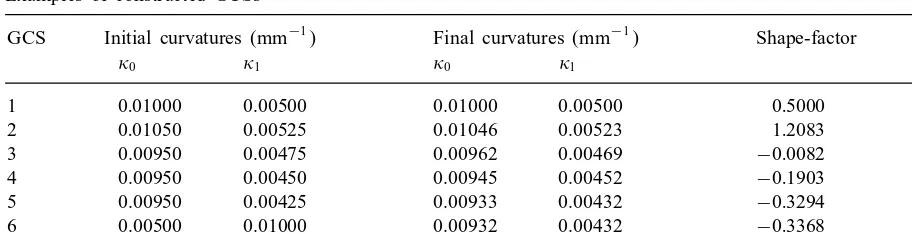
Table 1
Examples of constructed GCSs
GCS Initial curvatures (mm−1) Final curvatures (mm−1) Shape-factor Arc-length
0 1 0 1 (mm)
1 0:01000 0.00500 0.01000 0.00500 0:5000 100.0000
2 0:01050 0.00525 0.01046 0.00523 1:2083 99.9628
3 0.00950 0.00475 0.00962 0.00469 −0:0082 100.0410
4 0.00950 0.00450 0.00945 0.00452 −0:1903 100.0609
5 0.00950 0.00425 0.00933 0.00432 −0:3294 100.0798
6 0.00500 0.01000 0.00932 0.00432 −0:3368 100.0807
7 −0.01000 0.00500 0.00867 0.00179 −0:8449 100.2146
values for 1. Again, the algorithm behaves in a predictable manner with the nal curvatures varying
almost proportionally. It can be deduced therefore that the algorithm is stable with respect to small changes to the initial curvatures provided the curvature estimates are reasonable. The last two GCSs demonstrate that the algorithm is robust and can cope with ill-conditioned span data. Ideally, the curvature prole needs reecting for GCS 6 and the sign of 0 needs changing for GCS 7.
Finally it should be remarked that for all the well-conditioned sets of span data, the extra shape control of the GCS enables the specied end curvatures to be matched within 2%, and the discrep-ancies are not detectable by eye. However the discrepdiscrep-ancies using a Cornu spiral would be much larger and visible in GCSs 4 and 5.
7. Conclusions
This paper has introduced the generalised Cornu spiral. In particular, the curvature prole of a Cornu spiral has been generalised from a linear to a rational linear function of arc-length. This gives one additional degree of freedom that can be used to control the shape of the curve. It has been demonstrated that the GCS provides a one-parameter family of solutions to the simplied span generation problem when the curvature constraint is relaxed.
The algorithm described in this paper has been extended to three dimensions by considering two planar views of the span data and constructing GCSs in each of these planes. When combined using parallel projections, the resulting space curve is expected to be a quality curve since the two planar GCSs are themselves quality curves. The algorithm works well in practice provided the span data is nearly planar, that is, the torsion prole is insignicant. However, no consideration has been given to the resulting curvature prole on the three-dimensional GCS due to the construction based approach rather than an analytic one.
Acknowledgements
The authors are pleased to acknowledge the support of the UK’s Engineering and Physical Sci-ences Research Council (GR/K 31268). The rst author would like to express his gratitude to The University of Science Malaysia for a study grant under the Academic Sta Higher Education Scheme that allowed him to complete his Ph.D. at The University of Birmingham.
Appendix. Reection of the curvature prole
It is proved that if (−1=2)(1=2−tan−1(y1=x1))¿0, then reection of the curvature prole about
1=S, i.e., ′(s) = 21=S−(s), gives (′−1=2)(1=2−tan−1(y1=x1))¡0, where ′ corresponds to
the GCS with the reected curvature prole. In essence, it is proved that (−1=2)(1=2−′)¿0,
and hence the desired result follows immediately.
Consider the three curvature proles a(s) =(s), b(s) =1=S and c(s) = 21=S −(s) each
dened over 06s6S, where S ¿0. a(s) is the original and c(s) the reected curvature prole.
b(s) is a constant curvature prole corresponding to the mean tangent rotational angle [11]. Recall
the denition of , −=2¡ ¡=2, from Eq. (14), and let a, b and c correspond to the curves
with a(s), b(s) and c(s) respectively. Sincea=, b=1=2 and c=′, then (−1=2)(1=2−
′)¿0 if, and only if, (
a−b)(b−c)¿0.
For convenience, let fa(t) =
Rt
0a() d, fb(t) = Rt
0b() d and fc(t) = Rt
0c() d, then there
are four cases to consider to complete the proof of (a−b)(b−c)¿0, namely
(i) −=2¡ fa(t)¡ fb(t)¡ fc(t)60;
(ii) −=2¡ fa(t)¡ fb(t)60¡ fc(t)¡=2;
(iii) −=2¡ fa(t)¡0¡ fb(t)¡ fc(t)¡=2;
(iv) 06fa(t)¡ fb(t)¡ fc(t)¡=2:
The rst two cases are proven here and then the other two follow mutatis mutandis.
(i) −=2¡ fa(t)¡ fb(t)¡ fc(t)60:
Let t ¿0, then 0¡ cosfa(t)¡ cosfb(t)¡ cosfc(t) and sinfa(t)¡ sinfb(t)¡ sinfc(t)60, since
the cosine function is positive, the sine function is negative and both functions are strictly increasing in (−=2;0]. Hence, 0¡ cosfa(t)¡ cosfb(t)¡ cosfc(t) and sinfa(t)¡ sinfb(t)¡ sinfc(t)60 for all t ¿0. This implies, since S ¿0, that
0¡
Z S
0
cosfa(t) dt ¡
Z S
0
cosfb(t) dt ¡
Z S
0
cosfc(t) dt
and
Z S
0
sinfa(t) dt ¡
Z S
0
sinfb(t) dt ¡
Z S
0
and hence
RS
0 sinfa(t) dt RS
0 cosfa(t) dt
¡
Rs
0 sinfb(t) dt RS
0 cosfb(t) dt
¡
RS
0 sinfc(t) dt RS
0 cosfc(t) dt
60;
i.e., tana¡ tanb¡ tanc60. Since tan is strictly increasing in (−=2;0], then a¡ b¡ c
and (a−b)(b−c)¿0.
(ii) −=2¡ fa(t)¡ fb(t)60¡ fc(t)¡=2:
Lett ¿0, then 0¡ cosfc(t) and 0¡ sinfc(t). Hence, 0¡cosfc(t) and 0¡sinfc(t) for all t ¿0.
This implies 0¡ RS
0 cosfc(t) dt and 0¡ RS
0 sinfc(t) dt, and hence 0¡ RS
0 sinfc(t) dt= RS
0 cosfc(t) dt,
i.e., 0¡ tanc. Now, tana¡ tanb60 from case (i), and therefore it follows that tana¡tanb
¡ tanc. Since tan is strictly increasing in (−=2;=2), then a¡ b¡ c and (a−b)(b−
c)¿0.
References
[1] J.A. Adams, The intrinsic method for curve denition, Comput.-Aided Des. 7 (1975) 243 – 249. [2] J.M. Ali, Geometric control of planar curves, Ph.D. Thesis, The University of Birmingham, UK, 1994.
[3] A.A. Ball, CAD: Master or Servant of Engineering? The Mathematics of Surfaces VII, T. Goodman, R. Martin (Eds.), Information Geometers, Winchester, UK, 1997, pp. 17 – 23.
[4] J.V. Ball, Generation of smooth curves and surfaces, Ph.D. Thesis, The University of Birmingham, UK, 1997. [5] G. Darboux, Lecons sur la theorie generale des surfaces, vol. I, Gauthier-Villars, Paris, 1887.
[6] R.T. Farouki, Pythagorean-hodograph quintic transition curves of monotone curvature, Comput.-Aided Des. 29 (1997) 601– 606.
[7] D.S. Meek, D.J. Walton, Clothoid spline transition spirals, Math. Comp. 59 (1992) 117 – 133.
[8] D.S. Meek, D.J. Walton, Approximating quadratic NURBS curves by arc splines, Comput.-Aided Des. 25 (1993) 371– 376.
[9] A.W. Nutbourne, R.R. Martin, Dierential Geometry Applied to Curve and Surface Design, Ellis Horwood, Chichester, UK, 1988.
[10] A.W. Nutbourne, P.M. McLellan, R.M.L. Kensit, Curvature proles for plane curves, Comput.-Aided Des. 4 (1972) 176 –184.
[11] T.K. Pal, Mean tangent rotational angles and curvature integration, Comput.-Aided Des. 10 (1978) 30 – 34. [12] T.K. Pal, A.W. Nutbourne, Two-dimensional curve synthesis using linear curvature elements, Comput.-Aided Des.
9 (1977) 121 – 134.
[13] A. Schechter, Synthesis of 2D curves by blending piecewise linear curvature proles, Comput.-Aided Des. 10 (1978) 8 – 18.