isprs annals IV 2 W1 201 2016

(1)

A DATA STRUCTURE FOR PROGRESSIVE VISUALISATION AND EDITION OF

VECTORIAL GEOSPATIAL DATA

J. Gaillarda, b_{, A. Peytavie}a_{, G. Gesqui`ere}a

a

Univ Lyon, LIRIS, UMR 5205 F-62622, Villeurbanne, France b

Oslandia, France

KEY WORDS:3D, Visualisation, Web, Geospatial

ABSTRACT:

3D mock-ups of cities are becoming an increasingly common tool for urban planning. Sharing the mock-up is still a challenge since the volume of data is so high. Furthermore, the recent surge in low-end, mobile devices requires developers to carefully control the amount of data they process. In this paper, we present a hierarchical data structure that allows the streaming of vectorial data. Loosely based on a quadtree, the structure stores the data in tiles and is organised following a weight function which allows the most relevant data to be displayed first. The relevance of a feature can be measured by its geometry and semantic attributes, and can vary depending on the application or client type. Tiles can be limited in size (number of features or triangles) for the client to be able to control resource consumption. The article also presents algorithms for the addition or removal of features in the data structure, opening the path for the interactive edition of city data stored in a database.

1. INTRODUCTION

Virtual cities are an ever more growing research topic, with a great variety of applications for urban planning, routing, simula-tion or cultural heritage (Biljecki et al., 2015). Technical chal-lenges still remain, especially regarding the high amount of data in a virtual city model. To allow the best user experience, this data needs to be streamed. While there exist efficient methods for the progressive streaming of raster data, few satisfying solu-tions exist for vectorial data. Most of these solusolu-tions require a long preprocessing stage, where the data is organised, simplified or generalised and often duplicated. The result is generally a new dataset suitable only for visualisation that needs to be recomputed whenever the original data is modified.

An alternative to the costly generalisation of the geometry is the transmission of a subset of the data. In a lot of use cases, only a handful of features are of interest to the user. Transmitting and displaying only the most relevant data allows the user to rapidly access a view containing most of the information he needs at a low cost.

When transmitted from the server to the client, the city model’s geometries are usually not sent individually, but packed together in atile. With the surge in mobile devices, there is a need to control the amount of resources allocated to an application, and therefore the quantity of data within each tile. Since city models do not have a constant density, vectorial data has to be organised in hierarchical structures in order to have tiles of roughly the same size.

Being able to carry out geometrical operations or to edit the data opens up the use cases of virtual cities. For this purpose, hav-ing a shav-ingle model for both the visualisation and the storage of the data seems convenient. Furthermore, a unified model re-moves the need to duplicate the data (base model and visuali-sation model). With datasets covering larger and larger areas, exceeding the city scale, as well as existing in multiple temporal versions (Chaturvedi et al., 2015a), storage may well become an issue in the future.

The contributions of our paper are as follows:

• an efficient hierarchical structure for vectorial data allowing: – progressive loading of data based on a weight function – dynamic addition and removal of data

– compatible with rising exchange formats such as 3D-tiles (3D Tiles - Specification for streaming massive heterogeneous 3D geospatial datasets, 2016) • an architecture for visualising data from a geospatial database

featuring:

– fast deployment

– original storage format, suitable for 3D analysis The paper is organised as follows: we will review the state of the art in the fields of web 3D and virtual cities, then we will describe our data model and, in the next section, the detailed algorithms for creating and updating our data structure as well as ways of accessing the data. We will then present some results of our im-plementation of the model, both client-side with visual results of the progressive streaming and server-side with performance mea-surements. Finally, we will conclude and present leads for future works.

2. STATE OF THE ART

Progressive streaming of 3D geometries is a problem that has been addressed by numerous papers in the last 20 years (Hoppe, 1996). It is especially relevant nowadays, with web applications becoming so common and embedding 3D content thanks to We-bGL (Evans et al., 2014). The geospatial field is especially con-cerned by these works since it deals with a huge quantity of data. A lot of the research has already been done for terrain streaming (Lerbour, 2009), but streaming buildings and other city objects (roads, bridges, tunnels, etc.) is a much more recent topic.

The existing approaches for streaming 3D vectorial data can be classified in two main categories : generalisation on the one hand and progressive transmission on the other.

(2)

method for generating levels of details where each level is an in-dependent geometry: transitioning from one level of detail to the other requires the loading of a whole new object. (Mao, 2011) presents a variety of methods for creating simplified representa-tions of city models. (He et al., 2012) and (Guercke et al., 2011) generate multiple LoDs for building groups by generalising the footprint of the buildings.

Since its levels of details are independent, generalisation can pro-duce better quality approximations than other methods that use additive refinement as level of detail. Such methods fall within the progressive transmission class. Additive refinement is a de-sirable feature for web applications since data transmission is a frequent bottleneck. Progressive data structure may still have a cost, but it is usually far lower than that induced by generalisa-tion methods. (Ponchio and Dellepiane, 2015) presents a method for streaming high-quality meshes. Portions of the meshes are refined depending on the camera position.

Web city viewers often use very simple progressive loading meth-ods for buildings. A 2D grid manages the loading of data in (Chaturvedi et al., 2015b), (Gesquiere and Manin, 2012) or (Gail-lard et al., 2015). While its simplicity can be attractive for web applications, the visual result is unsatisfactory: data is loaded non-uniformly, in chunks. Areas of interest may be loaded last since only geometric metrics are used to define which grid tiles are loaded: only the camera position counts, not the nature of the data.

Hierarchical data structures are popular in the geospatial field, since they are well suited for data of varying scale. (Su´arez et al., 2015) presents a globe application, where the use of a quadtree enables constant resource usage. However, this only works for regularly meshed tiles, where each tile has the same number of triangles. Furthermore, vectorial data stored in quadtrees often overstep the boundary of the tiles, making them somewhat com-plex to manage. In geospatial databases, r-trees (Guttman, 1984) are often used to index the data. While it offers quick access to the features and solves the problem of overstepping features, it is not suitable for progressive streaming: all the features are stored at the same depth, in the leaves of the tree (there is no hi-erarchy of features), and features of the same leaf tile are always close to one another, meaning that a progressive loading based on this structure will be non-uniform and chunky, similarly to a grid. (Christen, 2016) uses a bounding volume hierarchy to or-ganise 3D buildings, but doesn’t provide any insight on how the BVH should be built. In the ray tracing field, common methods to build bounding volume hierarchies rely on heuristics such as SAH (Wald, 2007). However, constructing BVHs in this manner does not allow the user to control the depth in which the objects are in the BVH.

Most of recent approaches are based on a strong relation between the client and its dedicated server. For several years, the Open Geospatial Consortium has been proposing standards to facili-tate communication between different servers and clients. Recent works (3D Portrayal Interoperability Experiment, 2016) tend to propose a 3D portrayal specification, that may be followed in an implementation of this paper’s method, in order to provide a non-intrusive solution server-side.

In this paper, we present a progressive transmission method based on a data structure which allows a uniform loading of features over the whole extent of a scene, that takes into account not only the spatial position of the features, but also their semantic infor-mation. This produces a partial representation of a city composed of the most relevant features without the need to generate a new dataset or to download redundant data.

3. DATA MODEL

In this section, we will present our solution for storing and edit-ing a geospatial dataset. A description of the data structure is presented in figure 1. This datasetSis defined as a collection of featuresF. A featureFiis a 3D geometry to which is assigned

a number of semantic attributesAi. For instance, a feature could

be a building with attributes such as height, energy consumption, etc. A feature could also be a bridge with its name and date of construction as attributes.

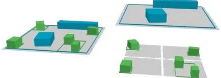
Figure 1: The bounding box hierarchy (left) and an exploded view of it (right).

Our goal is to retrieve data in chucks of similar sizes. Addition-ally, we wish to retrieve the most important data first. Since a city has variable density, we either need an irregular organisation of the data or a hierarchical data struture. In our case, hierarchi-cal data structures are preferable since they allow the ranking of data. Therefore, we store our data in a Bounding Box Hierar-chy (BBH): a tree where each node has a bounding box which strictly encloses all the underlying features (see figure 2). This is an advantage compared to the usual structures used for tiling cities (quadtrees or regular grids), where some features may over-step their tile’s boundaries and causes imprecisions in the loading of its features. In this paper, we use bounding boxes since our data has almost no verticality. In some cases, Bounding Volume Hierarchies (BVH) might be a better choice. The presented meth-ods work with both BBH and BVH with virtually no change.

The whole hierarchy Level 0 node Level 1 nodes

Feature Node Bounding Box

Underlying Quadtree Bounding Box

Figure 2: A 2D representation of the bounding box hierarchy structure.

Choosing a hierarchical data structure allows us to easily enable progressive loading: by storing features in the nodes of each level of the tree, the data will automatically be loaded progres-sively, starting from the topmost nodes down to the leaves. The higher the node is in the hierarchy, the more relevant it must be to the user’s visualisation. To quantify this relevance, each feature has an associated weight. We will discuss the computing of this weight in section 4.1.

(3)

deeper than those of sparse parts. This is not a problem: our main goal is to have tiles which have a similar weights and progressive loading, it is therefore natural that we have theses disparities.

In this paper, atileis the spatial aspect of anode, i.e. the bounding box and the features contained in a node.

There are various ways of limiting the number of features in a node. In the examples and algorithms of this paper, we define a maximum number of features per node, but it is also possible to set a maximum number of points or triangles per node. This is especially useful for low-end clients that need to control the amount of data they download or render. Using these more com-plex metrics (where the limiting property varies from feature to feature) raises the issue of packing the features into nodes in an optimal manner. This is a classic knapsack problem. We use a very simple approach, where as soon as a feature overfills a node, it is considered full. This solution offers satisfying results, further optimisation is left for future works.

Bounding box hierarchies (or bounding volume hierarchies) are a fairly common data model. Some exchange formats, most no-tably AGI’s 3D-tiles (3D Tiles - Specification for streaming mas-sive heterogeneous 3D geospatial datasets, 2016), already support these kind of structures, assuring compatibility with standard-compliant web clients. The specificity of our method, namely the way we order the features inside the hierarchy, takes place on the server and is completely transparent for the client.

4. DATA PROCESS

In this section, we will describe methods for initialising, editing and accessing the data of the BBH. An overview of the processes the BBH undertakes is shown in figure 3. Detailed algorithms are available in the appendix.

Original scene

Classification

Add Remove

Feature Tile Bounding Box Level-0 objects Level-1 objects

Figure 3: Manipulation data with our proposed structure: classi-fication, addition and removal of data.

4.1 Classification

The classification of the features in the bounding box hierarchy is based on the weight associated to each feature. This weight is determined by a functionfbased on the feature’s geometryGi

and semantic attributesAi:W(Fi) =f(Gi, Ai).

The choice of weight function depends on the target application. The most important features for the application should get the highest weight. For example, in a simple city visualisation appli-cation, the biggest buildings should be displayed first, and thus have a higher weight. If the application is focused on tourism, monuments should be favoured by the function. In section 4.4 we will present ways of creating and combining weight functions.

In the examples throughout this paper, for the sake of simplic-ity, we will use a purely geometric weight function based on the ground surface of a feature:W(Fi) =ground surf ace(Gi).

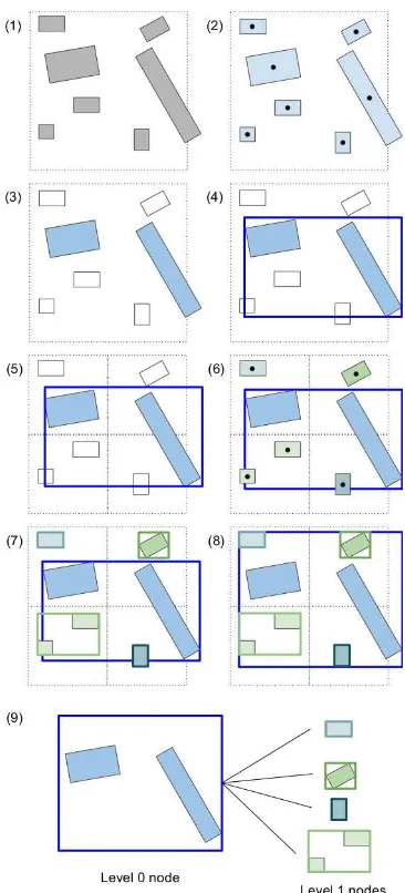
Figure 4: Initialisation algorithm for n = 2. (1) Initial state. Dashed square is the initial quadtree tile, covering the extent of the scene. (2) Assigning features to the node. (3) Selecting highest-weight features. (4) Computing bounding box. (5) Re-cursion, since all features are not assigned to a node yet. Creating child nodes using quadtree subdivision. (6) Assigning features to nodes. (7) Computing bounding boxes. (8) Adjusting parent bounding box. (9) The resulting structure.

Figure 4 goes through the classification process for a simple case. The algorithm is described hereafter. The numbers refer to the figure’s corresponding steps.

Initialisation (1):

• The extent of the scene (a bounding box which covers all the features) is defined. This is also the root of the quadtree upon which the selection process will be based. For large datasets, the extent can be cut into a grid where each grid tile will be the root of a quadtree;

• The features are sorted by descending weight, such that the first accessed features are always the ones with the highest weight;

• The maximum number of featuresnby tile is chosen.

(4)

Add thenfirst features to the node (3). Create the bounding based on these features (4). Divide the quadtree tile (5) and assign the remaining features to each of its children based on the position of their centroids (6). Repeat the process for each child, until no features are left (7).

Recursively adjust the bounding box of the nodes such as the par-ent node’s bounding box encloses its features and its children’s bounding box (8). The resulting structure is shown in (9).

4.2 Adding and Removing Features

Adding or removing data from the structure requires careful reor-ganisation to maintain the integrity of the database: the ordering of the features in accordance with their weight must be preserved, the maximum number of features per node must not be exceeded and the bounding boxes must be adjusted.

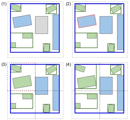
4.2.1 Addition The insertion of a feature (figure 5) requires finding the first node which fulfils the two following conditions:

• the node is not fullorthe weight of the new feature is be-tween the weight of the lowest and highest weight features of the node;

• the new feature’s centroid is inside the quadtree tile associ-ated to the node.

The quadtree tiles that contain the new feature’s centroid are tra-versed from top to bottom until a node that validates the first con-ditions is found.

The new feature is added to the node. If the node’s number of features exceedsn, the lowest weight feature of the node is re-moved and added to the child node. The process is repeated until the addition of a feature does not cause a node to be overfull.

Once the hierarchy has been reorganised, the bounding boxes of the altered nodes are recomputed.

(1) (2)

(3) (4)

Figure 5: Adding procedure. (1) Feature to add (in grey). (2) Find lowest weight feature (red border) of current tile. (3) Remove lowest weight feature from child tile and add it to the child tile in which it lies (red dashed border). (4) Recompute bounding boxes.

4.2.2 Removal Removing a feature (figure 6) from a node re-quires rebalancing the hierarchy. The removed feature of a node is replaced by the highest weight feature of its children. The child from which the feature was taken undergoes the same process, until the leaves of the tree are reached.

The bounding boxes are then resized for each altered node.

(1) (2)

(3) (4)

Figure 6: Removal procedure. (1) Feature to remove (red border). (2) Find lowest weight child feature (red border). (3) Remove lowest weight child feature from child tile and add it to current tile. (4) Recompute bounding boxes.

4.3 Accessing the Data

We recommend storing the features in a spatial database on the server. The features are indexed by the identifier of the tile to which they belong. This allows the server to select very quickly the features that a client needs, as the client sends requests for specific tiles.

The client accesses the data by querying the tiles that are inside its field of view and match its desired precision. For this task, the client must know in advance the bounding box and the level of detail of each tile. We call refinement scheme the way each tile is subdivided into its child tiles, that is the number of child tiles and their bounding boxes.

There are two main ways of managing the transmission of the re-finement scheme. The rere-finement scheme of the whole structure can be sent on initialisation of the application, solving the issue once and for all. This has the advantage of allowing the client to query multiple levels of tiles if needed, but can slow the initiali-sation of an application if the dataset is large and has a lot of tiles. The alternative is to transmit the scheme progressively, along the features. When answering a tile query, the server sends both the features and the tile’s refinement scheme.

4.4 Creating a weight function

In this section, we will define guidelines for creating and com-bining weight functions. A weight function assigns to a feature a weight, represented as a floating point number between 0 and 1. The higher the weight, the more importance is attached to the feature.

F7!W(F),R![0..1]

Surface Weight A classification based on the 2D footprint of a building allows the largest buildings to be displayed first. It is a pertinent choice for visualisation applications since these build-ings are big enough to be seen from afar and can be used as land-marks for orientation purposes.

(5)

the dataset. Cities often have a few buildings that are very large in comparison to the others. To avoid the weight values of most of the buildings to be clumped up near 0 as a result, we recommend using a function that returns 0.5 for a building that has the average size. Here is such a function, withSthe surface,avgthe average surface of features in the data set andmaxthe maximum surface:

surf ace weight(F) = ( _S

2∗avg ifS < avg

1− S−max

2∗(max−avg) ifS >=avg

Attribute Weight Semantic attributes can be used as a classifi-cation method. As they vary wildly in nature, it is hard to define a precise guideline for these weight functions.

Combining Weight Functions We can combine weight func-tions to create new, more complex funcfunc-tions. To each function Wiis assigned an importance factorwi. The weighted arithmetic

mean of these functions form the new weight function.

W(F) =

For example, let’s combine into a functionWCthe surface weight

functionW1described above and an attribute weight functionW2 that returns 1 for red features, 0 for blue features. Forw1=w2=

1,WCwill be a function that first prioritises the red features, then

order features according to their ground surface. Forw1 = 1 andw2 = 0.5, WC will be a function that guarantees that the

red features will be displayed first only if their are larger than average. Figure 7 illustrates this example.

A B C D E

Figure 7: Different weight functions. Highest weight feature is on the left, lowest weight feature is on the right.(1) Surface weight. (2) Combined surface and attribute weight. w1 = w2 = 1. (3)Combined surface and attribute weight.w1= 1, w2= 0.5.

5. RESULTS 5.1 Implementation and performance

All the following results were obtained on an Intel c$CoreTM i5-4590 CPU @ 3.3GHz x 4, Nvidia GeForce GTX 970.

We implemented the algorithms for creating and manipulating our data structure in Python, using psycopg2 (psycopg2 - Python-PostgreSQL Database Adapter, 2016) to interact with a postgres

database (PosgreSQL - The world’s most advanced open source database., 2016). We use the postGIS extension to handle geospa-tial data (PostGIS - Spageospa-tial and Geographic Objects for Post-greSQL, 2016).

We tested our algorithms on a dataset of close to 30,000 features of the city of Lyon and a second dataset of 80,000 features of the city Montr´eal. Results for Montr´eal are written in parenthe-ses. The initial state of the database for our study was a postGIS database filled with the aforementioned data indexed by gid.

We chose a weight function that returns the area of the footprint of the building and a maximum of 50 features per tile. It took 6.1 (11.4) seconds to create our data structure. 1.3 (1.9) seconds were spent fetching the data from the database and computing the weight of each feature, 4.6 (8.9) seconds were spent updating the database with a new tile index. The remaining 0.2 (0.6) second was used to organise the data inside our structure.

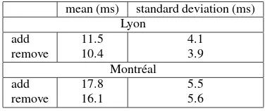
Adding and removing features from the database and updating the data structure is also fast. For the same database, which had 1165 tiles and up to 5 depth levels, each of these operations took barely more than 10 milliseconds (see table 1).

mean (ms) standard deviation (ms) Lyon

Table 1: Add and remove operations performance.

5.2 Test client

We use an Apache2 server combined with Python scripts to man-age the server-side processes.

Client-side, we visualise the data using Cesium (Cesium - We-bGL Virtual Globe and Map Engine, 2016). Our Javascript im-plementation features the progressive loading of buildings as in-tended by our data structure.

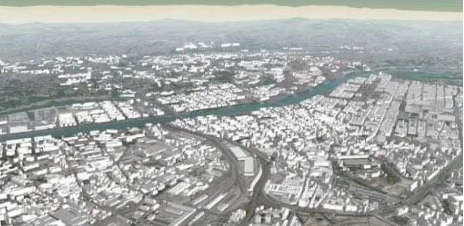
Figure 8: Screenshot of our web application based on Cesium. Buildings in red belong to level 0 tiles, those in orange to level 1 tiles, those in yellow to level 2 tiles and those in green to level 3 tiles.

(6)

Figure 9: Screenshot of our web application based on Cesium. In the foreground, most of the buildings are loaded, while only the most prominent are displayed in the background.

We limited the number of triangles loaded in the scene and com-pared the result for different loading methods. Figure 10 shows a comparison between our method, with a weight function based solely on the ground surface of the buildings, and a grid of 500m x 500m tiles.

We implemented different weight functions to observe the effect changing these functions has on the displayed scene:

W1(F) =surf ace weight(F) (1)

W2(F) =

surf ace weight(F) +is noteworthy(F)

2 (2)

is noteworthy(F) = (

1 ifFhas the noteworthy attribute 0 otherwise

(3)

W3(F) =

surf ace weight(F) +distance weight(F)

2 (4)

distance weight(F) =max(0,1−distance to rhone 500 ) (5)

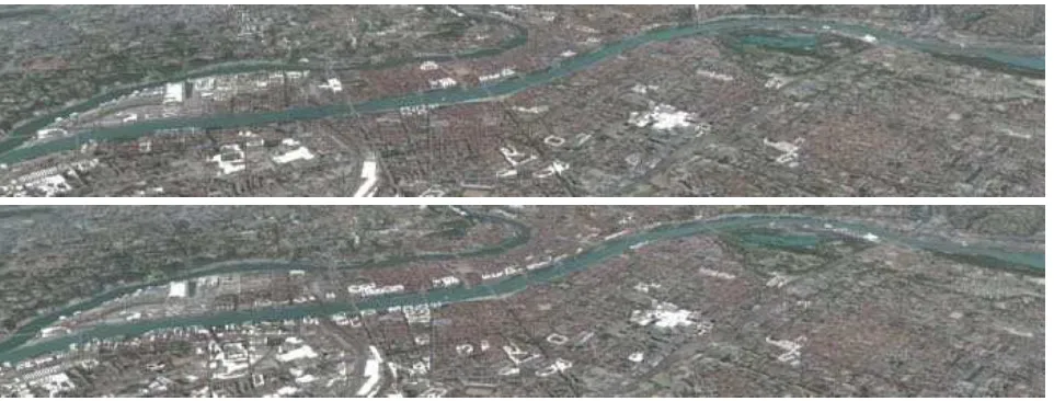
In figure 11, we see that more noteworthy buildings are loaded while usingW2instead ofW1. Figure 12 shows similar results, far more buildings are loaded next to the Rhˆone river whenW3is used.

5.3 Limitations

Changing the weight function requires the reprocessing of the full structure. It is however possible to have multiple indexes to pro-vide different classifications from which to choose.

A drawback of this data structure is that not all the loaded data will be in the camera’s field of view. Features are stored in each level of the hierarchy and the topmost tiles can be quite large. Therefore, if the camera does not cover the full extent of a tile, which is likely for the tiles that are high in the hierarchy, it is likely that some features will be loaded despite not being visible. A way to mitigate this problem is to have multiple level-0 tiles by cutting the original extent into a grid, as suggested in section 4.1.

Figure 11: Different weight functions and 500,000 triangles limit. The top image usesW1and the bottom oneW2. Red buildings are noteworthy.

6. CONCLUSION AND FUTURE WORKS

We have presented a novel data structure for the storage of vec-torial data. Its hierarchical nature allows the data to be easily streamed and is therefore suitable for web applications. More-over, features are ordered according to a weight function, making the first features to be loaded the most relevant ones. This prop-erty also means that if only a limited number of features can be loaded, due to limited processing power or storage, these features will be the most relevant ones for the current view.

(7)

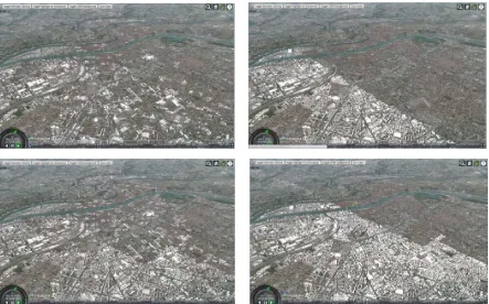
Figure 10: The scene loaded with our method, limited at 500,000 triangles (top left) and 1,000,000 triangles (bottom left). The scene loaded with a grid, limited at 500,000 triangles (top right) and 1,000,000 triangles (bottom right).

or removing features is fast, a few milliseconds, compared to the time it takes to create the hierarchy, which takes seconds.

We achieve better visual results sing our bounding box hierarchy construction method than using traditional data structures such as grids. Furthermore, thanks to the weight function, we allow semantic data to have an impact on visualisation. This can be used to create specific views for use cases by giving higher weight to features that have semantic attributes that are relevant to the use case.

Future works include adding support for geometric level of de-tail. Deeper levels of the hierarchy could be loaded with a lower geometric level of detail while top levels would be loaded at full detail.

Another improvement would be the possibility to combine differ-ent weight functions to generate a new structure on the fly, based on the classification of each function. This would allow the user to customise his view without needing to recompute the whole hierarchy.

A future improvement could be the use of new metrics to de-cide which tile needs to be refined. Traditionally, only geometric metrics like screen space error are used to choose which tiles of a hierarchical data structure have to be displayed. Choosing to load a tile not only for its position relative to the camera but also for the quantity of information it brings to the scene (see figure 13) would allow semantic information to play a bigger role in city viewing applications, and hopefully lead to a smoother experi-ence for the user.

ACKNOWLEDGEMENTS

This work has been supported by the french company Oslandia through the phd thesis of Jérémy Gaillard. CityGML data are provided byLyon metropoleandVille de Montréal. This research

Figure 13: An alternative way to handle feature loading. Level two tiles (in orange) are loaded despite being far from the camera because they have been found to bring more information to the scene.

was partly supported by the French Council for Technical Re-search (ANRT).

REFERENCES

3D Portrayal Interoperability Experiment, 2016. http://www. opengeospatial.org/projects/initiatives/3dpie. Re-trieved June 10, 2016.

3D Tiles - Specification for streaming massive heteroge-neous 3D geospatial datasets, 2016. https://github.com/ AnalyticalGraphicsInc/3d-tiles. Retrieved Mai 30, 2016.

Biljecki, F., Stoter, J., Ledoux, H., Zlatanova, S. and C¸ ¨oltekin, A., 2015. Applications of 3d city models: State of the art review. ISPRS International Journal of Geo-Information4(4), pp. 2842.

Cesium - WebGL Virtual Globe and Map Engine, 2016. http: //cesiumjs.org/. Retrieved June 10, 2016.

(8)

Figure 12: Different weight functions and 500,000 triangles limit. The top image usesW1and the bottom oneW3.

Chaturvedi, K., Yao, Z. and Kolbe, T. H., 2015b. Web-based exploration of and interaction with large and deeply structured semantic 3d city models using html5 and webgl. In: Bridging Scales - Skalen¨ubergreifende Nah- und Fernerkundungsmetho-den, 35. Wissenschaftlich-Technische Jahrestagung der DGPF.

Christen, M., 2016. Openwebglobe 2: Visualization of Complex 3D-GEODATA in the (mobile) Webbrowser. ISPRS Annals of Photogrammetry, Remote Sensing and Spatial Information Sci-encespp. 401–406.

Evans, A., Romeo, M., Bahrehmand, A., Agenjo, J. and Blat, J., 2014. 3d graphics on the web: A survey.Computers & Graphics 41(0), pp. 43 – 61.

Gaillard, J., Vienne, A., Baume, R., Pedrinis, F., Peytavie, A. and Gesqui`ere, G., 2015. Urban data visualisation in a web browser. In:Proceedings of the 20th International Conference on 3D Web Technology, Web3D ’15, ACM, New York, NY, USA, pp. 81–88.

Gesquiere, G. and Manin, A., 2012. 3D Visualization of Urban Data Based on CityGML with WebGL.International Journal of 3-D Information Modeling3(1), pp. 1–15.

Guercke, R., G¨otzelmann, T., Brenner, C. and Sester, M., 2011. Aggregation of lod 1 building models as an optimization problem. {ISPRS}Journal of Photogrammetry and Remote Sensing66(2), pp. 209 – 222. Quality, Scale and Analysis Aspects of Urban City Models.

Guttman, A., 1984. R-trees: A dynamic index structure for spatial searching.SIGMOD Rec.14(2), pp. 47–57.

He, S., Moreau, G. and Martin, J., 2012. Footprint-based 3d generalization of building groups for virtual city visualization. In: GeoProcessing2012: 4th International Conference on Ad-vanced Geographic Information Systems, Applications, and Ser-vices, pp. 177–182.

Hoppe, H., 1996. Progressive meshes. In: Proceedings of the 23rd Annual Conference on Computer Graphics and Interac-tive Techniques, SIGGRAPH ’96, ACM, New York, NY, USA, pp. 99–108.

Lerbour, R., 2009. Adaptive streaming and rendering of large terrains. Theses, Universit´e Rennes 1.

Mao, B., 2011. Visualisation and generalisation of 3D City Mod-els. PhD thesis, KTH Royal Institute of Technology.

Ponchio, F. and Dellepiane, M., 2015. Fast decompression for web-based view-dependent 3d rendering. In:Web3D 2015. Pro-ceedings of the 20th International Conference on 3D Web Tech-nology, ACM, pp. 199–207.

PosgreSQL - The world’s most advanced open source database., 2016. https://www.postgresql.org/. Retrieved Mai 30, 2016.

PostGIS - Spatial and Geographic Objects for PostgreSQL, 2016. http://postgis.net/. Retrieved Mai 30, 2016.

psycopg2 - Python-PostgreSQL Database Adapter, 2016.https: //pypi.python.org/pypi/psycopg2. Retrieved Mai 30, 2016.

Su´arez, J. P., Trujillo, A., Santana, J. M., de la Calle, M. and G´omez-Deck, D., 2015. An efficient terrain level of detail imple-mentation for mobile devices and performance study.Computers, Environment and Urban Systems52, pp. 21 – 33.

(9)

A. FULL ALGORITHMS

Notations:

• Na node of the tree;

• B(A)the bounding box of the node or the feature A; • C(N)the list of the child nodes of the node N; • P(N)the parent node of the node N;

• F(N)the list of the features of a node; • mF(N)the lowest weight feature of a node; • M F(N)the highest weight feature of a node;

• QB(N)the bounding box of the quadtree’s tile associated to the node N;

• Fa feature;

• W(F)the weight associated to the feature F;

• nthe maximum number of features that a node can contain.

A.1 Classification

1: forFinfeaturesdo