WIDE-AREA MAPPING OF FOREST WITH NATIONAL AIRBORNE LASER
SCANNING AND FIELD INVENTORY DATASETS
J.-M. Monnet a,*, C. Ginzler b, J.-C. Clivaz c a
Université Grenoble Alpes, Irstea, UR EMGR, 2 rue de la Papeterie - BP 76, F-38402 St-Martin-d’Hères, France – jean-matthieu.monnet@irstea.fr
b Swiss Federal Research Institute WSL, Zuercherstrasse 111, CH-8903 Birmensdorf, Switzerland - christian.ginzler@wsl.ch c
Canton du Valais - Arrondissement forestier du Valais Central – Rue Traversière 3, CH-1950 Sion, Switzerland - jean-christophe.clivaz@admin.vs.ch
KEY WORDS: Forest Inventory, Airborne Laser Scanning, Wide-area Mapping, Remote Sensing, Valais
ABSTRACT:
Airborne laser scanning (ALS) remote sensing data are now available for entire countries such as Switzerland. Methods for the estimation of forest parameters from ALS have been intensively investigated in the past years. However, the implementation of a forest mapping workflow based on available data at a regional level still remains challenging. A case study was implemented in the Canton of Valais (Switzerland). The national ALS dataset and field data of the Swiss National Forest Inventory were used to calibrate estimation models for mean and maximum height, basal area, stem density, mean diameter and stem volume. When stratification was performed based on ALS acquisition settings and geographical criteria, satisfactory prediction models were obtained for volume (R2=0.61 with a root mean square error of 47%) and basal area (respectively 0.51 and 45%) while height variables had an error lower than 19%. This case study shows that the use of nationwide ALS and field datasets for forest resources mapping is cost efficient, but additional investigations are required to handle the limitations of the input data and optimize the accuracy.
1. INTRODUCTION
In the past decade, many studies have demonstrated the potential of airborne laser scanning (ALS) for forest parameter mapping. The area-based approach combines the 3D description of vegetation by the ALS point cloud with field plot data in order to provide statistically calibrated, continuous maps of forest parameters (Naesset, 2002). This method has been tested in different forest contexts and with various acquisitions settings. It is now used for operational inventory with dedicated ALS and field campaigns in areas of around 100 km2. Besides, nationwide ALS acquisitions have been performed, mainly for topographic purposes, and field forest plot are routinely acquired for national or regional statistical monitoring of forest resources. These data can be used in a cost-effective way as inputs for the ALS-based mapping workflow (Hollaus et al. 2009, Nilsson et al. 2015) but have limitations as their acquisition is not designed for this purpose. In this case-study, we used nationwide ALS data and National Forest Inventory (NFI) data to derive forest parameters maps and identify the main limitations due to the input data.
2. MATERIAL AND METHODS
2.1 Study area
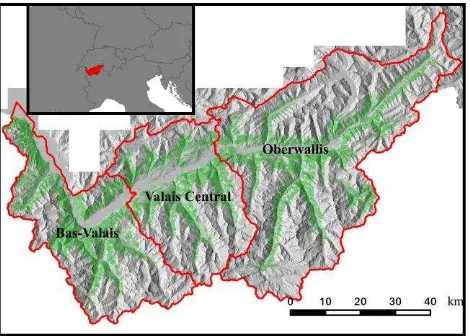
The study area is the Canton of Valais (Switzerland), with a total area of 522 450 ha. Forests are highly heterogeneous due to the elevation range (390 to 3550 m above sea level) and the steep topography (Figure 1). The Canton is divided in three arrondissements: Bas-Valais, Valais-Central and Oberwallis from west to east. Total forest area is 127 400 ha.
2.2 National forest inventory data
The objective of the Swiss NFI is to evaluate the current state
Figure 1. Map of study area
and monitor the dynamics of Swiss forests, based on a network of field sample plots. The sampling (Keller 2005) is based on a 1.4 km grid. Trees with a diameter at breast height (DBH) above 12 cm are inventoried up to a distance of 7.98 m from the grid node, and trees with DBH larger than 36 cm up to 12.62 m. From the tree-level measures, the Swiss Federal Institute for Forest, Snow and Landscape Research (WSL) derives plot-level forest parameters. In this study, mean height, maximum height, mean diameter, stem density, stem volume and basal area are considered.
Table 1 presents the statistics of the 688 plots located in the study area and measured in 2006 during the NFI III campaign. On 47 plots, no tree was measured. Height parameters are not calculated in 229 plots, due to sampling procedures. Forest parameters are highly variable, with volumes from 0 to 1439 m3/ha and basal areas from 1 to 139 m2/ha. This The International Archives of the Photogrammetry, Remote Sensing and Spatial Information Sciences, Volume XLI-B8, 2016
variability is due to both the heterogeneity of forests and to the small size of inventory plots (500 m2).
Mean
Table 1. Forest parameters statistics for the 688 NFI plots
NFI data result from a well-documented protocol and are available for the whole Swiss territory. However, their use for the calibration of estimation models from remote-sensing data has some limitations:
- the number of plots might not be sufficient for small surfaces (< 100 km2);
- the temporal difference between the field and remote sensing acquisitions;
- the spatial accuracy of the field plot position.
Strunk et al. (2012) showed that the minimum number of plots to avoid the over-estimation of model accuracy is 50. Regarding position accuracy of the NFI data in Valais, a study carried on a sample of 44 plots demonstrated a mean absolute position error of 4.6 m, with a standard error of 3.5 m. Previous studies showed that positions errors below 5 m have limited effect on models accuracy. But those results were obtained with larger plots and in more homogeneous forests (Gobbakken & Naesset 2009). Besides, when models are calibrated with shifted data, model error is rather over-estimated (Monnet & Mermin, 2014).
2.3 Airborne laser scanning data
ALS data was acquired for the whole Swiss territory between 2000 and 2008, for areas with altitude below 2000 m. ALS data are available as point clouds with X, Y and Z coordinates without other attributes. Point classification is not specified but the swissALTI3D digital terrain model (2-m resolution) was derived from this dataset. Flight metadata are limited to the following information: year and period of flight (spring / autumn / summer). The ALS point cloud in the study area was acquired in 2001 and 2005, and actually contains points up to an altitude of 2100 m. Average pulse density is around 0.5 m-2, which is sufficient for an area-based approach (Monnet et al. variations induced by those factors, stratum-specific models are calibrated. Strata are designed a priori to be more homogeneous
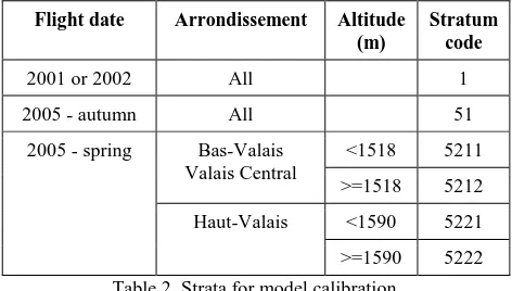
while containing a sufficient number of calibration plots. Six strata are considered depending on the flight date, arrondissement and altitude (Table 2).
Flight date Arrondissement Altitude (m)
Stratum code
2001 or 2002 All 1
2005 - autumn All 51
2005 - spring Bas-Valais Valais Central
<1518 5211
>=1518 5212
Haut-Valais <1590 5221
>=1590 5222
Table 2. Strata for model calibration
For model calibration, NFI plots located across ALS tiles
2.5 Metrics computation and modelling
The software FUSION (McGaughey, 2014) is used to compute ALS metrics. They are calculated on the one hand for the point cloud extracted for each NFI plot, based on their center considered as outliers and are also discarded. For each stratum and each forest parameter, only plots with positive values are used for calibration. The dependent variable is first transformed by a Box-Cox transformation of parameter λ to normalize its distribution. Then linear regressions with at most four independent variables are tested. The regression with the highest adj-R2 is retained as prediction model:
The following metrics are considered as candidate variables: Elev.minimum, Elev.maximum, Elev.mean, Elev.mode, Elev.stddev, Elev.variance, Elev.CV, Elev.IQ, , Elev.skewness, Elev.kurtosis, Elev.AAD, Elev.MAD.median, , Elev.MAD-mode, Elev.L1, Elev.L2, Elev.L3, , Elev.L4, Elev.L.CV, Elev.L.skewness, Elev.L.kurtosis, , Elev.P01, Elev.P05, Elev.P10, Elev.P20, , Elev.P25, Elev.P30, Elev.P40, Elev.P50, , Elev.P60, Elev.P70, Elev.P75, Elev.P80, , Elev.P90, Elev.P95, Elev.P99, Canopy.relief.ratio, Elev.quadratic.mean, Elev.cubic-mean, Percentage.all.returns.above.2.00, Percentage.all.returns-above.mean, Percentage.all.returns.above.mode. The altitude extracted from the swissALTI3D digital terrain model is also used as candidate variable.
Once the models are calibrated, parameter estimates
y
~
are obtained by applying model coefficients to the selected ALS metrics and applying the Box-Cox inverse transformation:
with var the variance of model residuals.
2.6 Accuracy evaluation
In absence of validation data, accuracy assessment is performed by leave-one-out cross validation. The root mean square error (RMSE) and its coefficient of variation (CVRMSE) are computed:
values for plot i, and n is the total number of plots. The bias and the mean absolute error (MAE) are also calculated.
The Table 3 presents aggregated statistics of the models.
Table 3. Global accuracy statistics of prediction models
Approximately 418 NFI plots were used for model calibration of height variables, and 582 for the other variables. For height
Figure 2. ALS estimates plotted against field measures, symbol color refers to the different strata
ALS
variables and stem volume, models account for more than 61% of variability, even though the root mean square error remains important (47%). A similar error is obtained for basal area, but with a lower coefficient of determination (51%). Models for mean diameter and stem density have little relevance. No bias is significant.
Accuracies are lower than usual values found in the literature, where there are typically 5 to 10% for height variables, 20 to 30% for volume and basal area. In the nationwide study in Sweden (Nilsson et al. 2015), accuracies were 17.2 to 23.3% for stem volume, 15.0 to 18.3% for basal area and 6.2 to 9.7% for tree height. The heterogeneity of forest stands and of the ALS data in the Valais might explain the lower accuracies.
Graphical displays of results (Figure 2) show that models tend to overestimate small values and underestimate large values, whatever the forest parameter. This could be linked to a saturation of the ALS signal in highly stocked forest stands or to the effect of temporal and spatial shifts between field and airborne acquisitions.
3.2 Wall-to-wall mapping
The ALS metrics are calculated for each pixel of a 20-m resolution raster covering the whole study area. Each pixel is affected to the corresponding stratum depending on its ALS flight date, arrondissement and altitude, according to the same criteria as for the NFI plots. Stratum-specific models are then applied to compute the forest parameter estimates.
Extreme values are obtained due to ALS point outliers. Thresholds are applied to the final map to remove such artefacts. Moreover, pixels located outside the forest mask
defined by the “wooded area” reference shapefile are set to NULL.
3.3 Arrondissement-level accuracy
For each arrondissement, the mean value for stem volume and basal area are computed, from the NFI data alone, and from the ALS-derived maps.
From the n NFI plots located in a given area of interest, the mean M and the error E corresponding to the 95% confidence interval [M-E, M+ E] are computed as:
i IF Ny
n
=
M
1
;
n
σ
n
t
=
E
IF N0.975,
1
y (9)with t(0.975, n-1) the quantile 0.975 of a Student distribution with n-1 degrees of freedom, and σy the standard deviation of
the nIFN values.
From the N pixels contained in the same area, the synthetic regression estimator (SRE) defined by Breidenbach & Astrup (2012) can be calculated as:
jSRE
y
N
=
M
1
ˆ
(10)Altitudes higher than 2050 m are discarded, because the ALS coverage might be incomplete. ALS estimates are an indirect but comprehensive measure of the study area. While the uncertainty of the NFI estimate results from the sampling,
uncertainty of the ALS value is due to the model error. Indeed, models can be mis-specified if the calibration data are not representative of the area of interest. An arrondissement-level bias correction is introduced to compute the generalized regression estimator (GREG) by removing the arrondissement-level bias calculated on the n local NFI plots:
i iSRE
GREG
y
y
n
M
=
M
1
ˆ
(11)Its confidence interval is computed similarly to formula (9) by using the standard error of model residuals instead of σy. Table
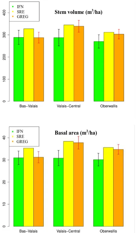
3 presents the results for the whole Valais. Results at the arrondissement level are displayed on Figure 3. The confidence intervals are smaller for the ALS-derived values, compared to those calculated from the NFI.
NFI SRE GREG
Volume (m3/ha) 281±19 326 307±14 Basal area (m2/ha) 30.6±1.8 36.2 34.2±1.4 Table 3. Mean volume and basal area estimates for the Valais
Figure 3. Mean volume and basal area for each arrondissement
IFN SRE GREG
Stem volume (m3/ha)
Basal area (m2/ha) IFN
SRE GREG
4. CONCLUSION
Existing methodology for the calibration of prediction models with airborne laser scanning was successfully implemented in the case of a wide-area mapping of forest variables. Using NFI sample plots and existing ALS datasets is cost-effective and the resulting maps have high added-value for local forest managers, despite higher errors compared to values obtained in specifically designed ALS-based inventories.
Regarding data acquisition, it seems important to have better meta data about acquisition parameters in order to be able to appropriately stratify the models in subsequent analysis. Besides, if statistical estimates have to be derived at some administrative level, attention should be paid to ensure homogeneous acquisition settings inside each administrative entity.
Temporal and spatial differences between field and remote sensing acquisitions still remain troublesome. Methods have been proposed to improve field data co-registration (Monnet & Mermin 2014), but they are not always applicable due to data quality. A better co-registration would benefit to many applications with remote sensing, so that special attention should be paid to GNSS geolocation during field measures. The effects of temporal difference have received little attention in the literature. Along with sampling issues, it might contribute to prediction models being mis-specified, and advanced statistical tools might be required to improve the estimation of domain-level attributes and of their associated uncertainty.
ACKNOWLEDGEMENTS
Irstea Grenoble, UR EMGR, is part of Labex OSUG@2020 (ANR10 LABX56).
REFERENCES
Breidenbach, J., Astrup, R. 2012. Small area estimation of forest attributes in the Norwegian National Forest Inventory. European Journal of Forest Research, 131, pp. 1255-1267.
Gobakken, T., Næsset, E. 2009. Assessing effects of positioning errors and sample plot size on biophysical stand properties derived from airborne laser scanner data. Canadian Journal of Forest Research, 39, pp. 1036-1052.
Keller, M. 2005. Schweizerisches Landesforstinventar. Anleitung für die Feldaufnahmen der Erhebung 2004–2007.
Hollaus, M., Dorigo, W., Wagner, W., Schadauer, K., Höfle, B., Maier, B. 2009. Operational wide-area stem volume estimation based on airborne laser scanning and national forest inventory data. International Journal of Remote Sensing, 30, pp. 5159– 5175.
McGaughey, R. J. 2014. FUSION/LDV: Software for LIDAR data analysis and visualization - Fusion version 3.42.
Monnet, J.-M., Chirouze, É., Mermin, É. 2015. Estimation de paramètres forestiers par données LiDAR aéroporté et imagerie satellitaire RapidEye - Étude de sensibilité. Revue Française de Photogrammétrie et Télédétection, 211-212, pp. 71-80.
Monnet, J.-M., Mermin, É. 2014. Cross-Correlation of diameter measures for the co-registration of forest inventory plots with airborne laser scanning data. Forests, 5, pp. 2307-2326.
Næsset, E. 2002. Predicting forest stand characteristics with airborne scanning laser using a practical two-stage procedure and field data. Remote Sensing of Environment, 80, pp. 88–99.
Nilsson, M., Nordkvist, K., Jonzén, J., Lindgren, N., Axensten, P., Wallerman, J., Egberth, M., Larsson, S., Nilsson, L., Eriksson, J., Olsson, H. 2015. A nationwide forest attribute map of Sweden derived using airborne laser scanning data and field data from the national forest inventory. In: Proceedings of Silvilaser 2015, pp. 211-213.
Pu, X., Tiefelsdorf, M. 2015. A variance-stabilizing transformation to mitigate biased variogram estimation in heterogeneous surfaces with clustered samples. In: Proceedings of the 13th International Conference on GeoComputation.
Strunk, J., Temesgen, H., Andersen, H. E., Flewelling, J. P., Madsen, L. 2012. Effects of lidar pulse density and sample size on a model-assisted approach to estimate forest inventory variables. Canadian Journal of Remote Sensing 38, pp. 644-654.