COEVRAGE ESTIMATION OF GEOSENSOR IN 3D VECTOR ENVIRONMENTS
A. Afghantoloee a *, S. Doodman a, F. Karimipour a, M. A. Mostafavi b
a Department of Surveying and Geomatic Engineering, College of Engineering, University of Tehran, Tehran, Iran (a.afghantoloee, s_Doodman, fkarimipr)@ut.ac.ir
b Center for Research in Geomatics, Department of Geomatics, University of Laval, Quebec, Canada [email protected]
KEY WORDS: geosensor deployment, WSNs, geosensor coverage, vector data model, DSM
ABSTRACT:
Sensor deployment optimization to achieve the maximum spatial coverage is one of the main issues in Wireless geoSensor Networks (WSN). The model of the environment is an imperative parameter that influences the accuracy of geosensor coverage. In most of recent studies, the environment has been modeled by Digital Surface Model (DSM). However, the advances in technology to collect 3D vector data at different levels, especially in urban models can enhance the quality of geosensor deployment in order to achieve more accurate coverage estimations. This paper proposes an approach to calculate the geosensor coverage in 3D vector environments. The approach is applied on some case studies and compared with DSM based methods.
* Corresponding author.
1. INTRODUCTION
Geosensors are tiny and ingenious devices that collect data about their nearby area, and are capable of communicating with each other. They are usually deployed in a wireless network to monitor and collect physical and environmental information such as motion, temperature, humidity, pollutants, and traffic flow in a given area (Romer and Mattern, 2004) . The information is then communicated to a processing center, where they are integrated and analyzed for different applications (Ghosh and Das, 2006). Capturing information of the environment is an important function of Wireless geoSensor Network (WSN) applications.
A geosensor covers only a certain region, which depends on the sensing and communicating range (limited by signal amplitude) as well as the environment conditions such as visibility (limited by obstacles). The total area covered by a WSN is obtained from the union of the regions covered by individual sensors. Efficient deployment of geosensors in a WSN is an important issue that affects the coverage as well as communication between sensors (Argany et al., 2011). The coverage problem in WSN is studied intensively in last decades. Several optimization methods (i.e., global or local, deterministic or stochastic, etc.) have been proposed to detect and eliminate coverage holes and hence increase the coverage of geosensor networks. Some methods use general optimization techniques, while some others consider the problem as a geometric issue and use tools from computational geometry (Karimipour et al., 2013). The key point of all deployment optimization algorithms, is determining the coverage of an individual geosensor.
The coverage problem is classified into target- and area-based coverage: In some of WSN applications, detecting the target points such as building, doors, flags and boxes are desired, while in others the aim is detection of the mobile target points like intruders (Guvensan and Yavuz, 2011). Covering the target points, instead of the whole area, is concerned in the target-based coverage problem, whose purpose is to achieve the maximum number of target points that have been covered. In target-based coverage, any target must be covered by at least
one sensor, or k sensors in some applications for the sake of certainty (Kumar et al., 2004). A main issue here is presence of obstacles, which has not been considered in most of the current studies (Li et al., 2003). An exception is the effort to consider the obstacles in target-based coverage to compute the best coverage path between two points in 2D environments (Roy et al., 2007), where the visibility graph (Welzl, 1985), as an standard structure, has been used for evaluating the intervisibility between the geosensors and targets.
On the other hand, in the area-based coverage problem, which is the concern of this paper, the objective is to obtain the maximum region covered by geosensors, and is usually evaluated as the ratio of the covered area to the whole area (Huang and Tseng, 2005). The area-based coverage calculation methods are classified into: (i) the methods that consider a raster environment (Akbarzadeh et al., 2013; Argany et al., 2012; Cortés et al., 2004), which are limited by the spatial resolution; and (ii) the methods that model the environment as a vector dataset (Ghosh and Das, 2006; Guvensan and Yavuz, 2011; Ma et al., 2009; Wang and Cao, 2006, 2011), which have been mostly proposed for 2D spaces and do not consider the earth topography and human-made obstacles. Furthermore, the sensing models (i.e., binary or probabilistic, omnidirectional or directional, etc.) significantly affect the coverage estimation. In this paper, we propose an approach to determine the coverage of a geosensor with directional sensing model in a 3D vector environment. To the best of our knowledge, there has been no solution for this case in the literature. The visibility calculation in our approach is a vector extension of the
pixel-based painter’s algorithm (De Berg et al., 2000), which draws each object onto a projection plane, and those parts of the objects that are not obscured by others are extracted.
of the DSM models. Finally, section 6 concludes the paper and contains ideas for future work.
2. ESTIMATION OF A SENSOR COVERAGE IN AREA-BASED METHODS
The area-based methods to estimate the sensor coverage are classified into raster and vector methods, both consider the two parameters distance and angle ranges for evaluating the coverage. In 2D raster methods (Figure 1.a) a pixel q is covered by a sensor S with the distance and angles ranges of (0, Rs) and
However, the covered area in 2D vector is simply calculated as (Figure 1.b):
Figure 1. 2D coverage estimation: (a) raster model (gray pixels are covered by the sensor S); (b) vector model (gray region is
covered by the sensor S)
The methods can be simply extended to support presence of obstacles in the environment: In raster model, the line connecting the pixel and the sensor is also checked against intersection with the obstacle pixels. In vector model, the regions behind the obstacles are extracted through connecting the sensor to the vertices of the obstacles.
In the 3D raster model, coverage estimation considers not only distance and angle ranges, but also the visibility between the sensor and pixels are of the same importance because of presence of the obstacles and the terrain topography (Figure 2):
S
The visibility between the sensor and pixels are checked by the line of sight (LoS) method (Seixas et al., 1999).
Figure 2. 3D coverage estimation in raster model (red pixels are not covered by the sensor S)
In the next section, we propose a method for geosensor coverage estimation for 3D vector models, which to the best of our knowledge has not been considered so far.
3. THE PROPOSED METHOD FOR CALCULATING COVERAGE IN 3D VECTOR SPACES
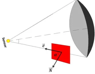
This section describes the proposed method for calculating the geosensor coverage in 3D vector spaces. As Figure 3 shows, we project the area covered by a directional sensor on a plane, called perspective plane, on which the sensing region of the geosensor is projected as a circle, called perspective circle, regarded as geosensor field of view.
Figure 3. Perspective plane and circle
To calculate the area covered by the geosensor, the following steps are performed, which are described in the next subsections:
1. Elimination of the back-face polygons
2. Elimination of the polygons lie on the back side of the perspective plane
3. Elimination of the polygons lie outside the distance range
4. Projection of the polygons on the perspective plane and overlaying them
5. Transformation of the projected polygons into their own 3D polygon planes
3.1 Elimination of the back-face polygons
polygon to the sensor. The normal of a convex polygon is simply calculated by using the first three vertices of the polygon as follows: Blinn and Newell (1976), who calculated the components Nx, Ny and Nz of the normal vector N as follows: normal of a non-convex polygon, but it is also provides the best estimation of the normal of non-planar polygons.
Given e is the vector toward the geosensor from a polygon and
N is the normal vector of that polygon, if e.N 0, then that polygon is called back-face and is not covered by the sensor, and thus is eliminated (Figure 4).
Figure 4. Elimination of the back-face polygons through the sign of the vector Ne.
3.2 Elimination of the polygons lie on the back side of the perspective plane
Since we consider a directional sensor, the polygons lie on the back side of the perspective plane will not be covered. As shown in Figure 5.a, to eliminate such polygons, the vectorse
toward all of the polygon’s vertices from the projected geosensor S are calculated. If the angles between the geosensor direction vector (ds
) and every single of the vectors are less than 90◦, this polygon is fully located in front of the perspective plane (e.g., polygon A in Figure 5.a). If all of these angles are bigger than 90◦, this polygon fully lies on the back side of the perspective plane (e.g., polygon B in Figure 5.a). If some angles are less and some are bigger than 90◦, the portion of the polygon that lies on the back side of the perspective plane must be calculated and eliminated (e.g., polygon C in Figure 5).
Figure 5. Elimination of the polygon B lies on the back side of the perspective plane. The portion of the polygon C that lies on
the back side of the plane is eliminated.
3.3 Elimination of the polygons lie outside the distance If all diss are smaller than Rs, the polygon lies inside the sphere (e.g., polygon B in Figure 6). In the case of intersection (e.g., polygon C in Figure 6), some diss are bigger and some are smaller than Rs, and the portion of the polygon that lies outside the sphere must be eliminated.
Figure 6. Elimination of the polygon A lies outside of the sensor distance range. The portion of the polygon C that lies
outside of the distance range is eliminated.
3.4 Projection of the polygons on the perspective plane and overlaying them
The polygons passed the above examinations are projected on the perspective plane according to the perspective geometry (Hoiem et al., 2008). As illustrated in Figure 7, the polygons projected in the 2D perspective plane are classified into:
The polygons that fall entirely within the perspective circle and are considered as "visible" (e.g., polygons A and B);
The polygons that are totally located outside the perspective circle, i.e., are out of the visible area of the geosensor.
through computing their intersection with the perspective circle (Figure 8).
Figure 7. Classifying the projected polygons on the perspective plane respect to their position in the perspective circle
Having the visible sections of each polygon calculated, they must be checked against other polygons to find the portion that is not obscured by other polygons. For this aim, any polygon is overlaid by other polygons according to depth sorting (Foley and Van Dam, 1982) to make sure that all of the polygons are behind it (Figure 8). The overlay is applied according to the overlying vector method presented by Leonov (2004).
The depth sorting algorithm sorts the polygons in order, from the furthest to the nearest respect to the geosensor vision. There are two solutions for depth sorting: (1) checking one of the intersection points between the two projected polygons and determining which depth is closer; and (2) Binary Space Partitioning (BSP) method extended to 3D space by Naylor (1990), which is a predefined process that creates a tree structure for capturing some relative depth information between polygons.
Figure 8. Overlaying the polygons with the perspective circle and together
3.5 Transformation of the projected polygons into their own 3D polygon planes
The projected polygons resulted from the above overlay process, are finally transformed into their own 3D polygon planes as the polygons covered by the sensor. For simplicity in the area computations, the polygons are first triangulated and then transformed (Figure 9). To compute the area of these triangles in the 3D space, the following formula is used:
) ,
cross( 2 1
2 3 1
2 v v v
v
Ar ea (7)
(a) (b)
Figure 9. (a) Converting the polygons to triangles; (b) Transformation of the triangles into their own 3D polygon
planes
The pseudo-code of the proposed approach is as follows:
Input: A set of 3D polygons P = {P1, …, Pn} that model the
3D environment
A geosensor node S and its position, direction, sensing range and field of view
Output: The region sensed by the geosensor S
1. Sort the 3D polygons {P1, …, Pn} descending based
on their distance to the geosensor (depth sorting) 2. Create an empty list L
3. For each sorted Pi
4. If Pi is located in front of S and within the distance range of it
5. PP← Projection of Pi on the perspective plane of S 6. V ← The portion of PP that fall within the
perspective circle of S 7. For each elements li in L 8. li = li–V
9. Insert V into L
10. T← Conversion of L to triangles
11. Transform T to 3D space and calculate the area
4. IMPLEMENTATION RESULTS
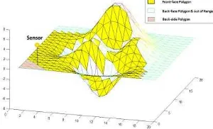
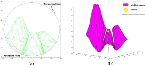
The proposed approach was implemented and applied on two case studies. In the first case, the peaks function as a simulated 3D environment was considered, and a 4-meter-high geosensor with 90° field of view in both vertical and horizontal directions was placed (Figure 10). Figure 11 illustrates the perspective view and the area covered by the geosensor, which is 68.98 m2.
(a) (b)
Figure 11. Calculating the coverage of the geosensor of Figure 10 (a) The perspective view; (b) The area covered by the
geosensor
A CityGML dataset was also used as another case study (Figure 12), where a geosensor with direction of [1, 1, -1] and 90° of field of view is considered. In CityGML, a 3D vector model consists of objects such as buildings, which per se are composed of a series of polygons, in a 3D space. Figure 13 illustrates the steps to calculate the area of the region covered by the geosensor, which is 143231.729 m2.
Figure 12. The sample CityGML dataset
(a) (b) (c)
Figure 13. (a) The polygons located in front of the sensor and within its sensing range; (b) The perspective view of the polygons visible by the sensor; (c) 3D polygons visible by
the sensor
In order to examine and compare the performance of the proposed approach with the raster-based methods, a CityGML dataset of LoD2 (including the buildings, terrain topography and trees) as vector model (Biljecki et al., 2014) and a DSM with the spatial resolution of 2m as raster model of the same region were considered (Figure 14). In the raster case, the DSM model of the region with other spatial resolutions was also tested to evaluate the effect of the resolution on the accuracy of the results. A geosensor with the distance range of 35m and angle range of 90◦ was placed at the point (100, 140, 20) and with the direction of [1, 1, -1].
(a) (b)
Figure 14. (a) The CityGML model; (b) DSM model with the spatial resolution of 2m
Figures 15 and 16 respectively illustrate the results of the CityGML and DSM models. The CityGML model considers the details of the environment (e.g., walls of the buildings and oblique planes) in the visibility analysis, whereas the DSM model only takes the roof of the buildings into account.
(a) (b)
Figure 15. (a) The perspective view of geosensor; (b) The area covered by the geosensor in CityGML model
On the other hand, in the case of DSM model, the accuracy of the coverage estimation improves with increasing the spatial resolution of the model (Figures 16 and 17), but the computation load also dramatically increases. While the CityGML model produces an accurate model with an acceptable accuracy and in a reasonable time.
(a) (b)
Figure 16. DSM model of the spatial resolution of (a) 2m; (b) 0.2m
5. CONCLUSIONS
This paper proposed an approach to determine the coverage of a geosensor with directional sensing model in a 3D vector environment. By recent advances in spatial information collection and increasing data accuracy and quality of spatial data, such as CityGML, this improvement seems inevitable. The approach was described and its implementation results for some case studies were presented. The results certify the beauty of the approach. On the other hand, comparing the results provided by the proposed and raster-based models showed that the coverage estimation is more accurate in the proposed vector-based method, as it considers the details of the environment (e.g., walls of the buildings and oblique planes) in the visibility analysis.
In future, we plan to use the proposed approach in various WSN deployment optimization methods in order to see how it affects the final placement. We also intend to exploit the approach in the k-coverage sensor problem.
6. ACKNOWLEDGEMENT
The authors would like to deeply appreciate Filip Biljecki for providing the CityGML data, without which the implementations and comparisons could not have been performed.
REFERENCES
Akbarzadeh, V., Gagne, C., Parizeau, M., Argany, M., Mostafavi, M.A., 2013. Probabilistic Sensing Model for Sensor Placement Optimization based on Line-of-sight Coverage. IEEE Transactions on Instrumentation and Measurement 62, 293-303.
Argany, M., Mostafavi, M.A., Akbarzadeh, V., Gagné, C., Yaagoubi, R., 2012. Impact of the quality of spatial 3D city models on sensor networks placement optimization. GEOMATICA 66, 291—305.
Argany, M., Mostafavi, M.A., Karimipour, F., Gagné, C., 2011. A GIS Based Wireless Sensor Network Coverage Estimation and Optimization: A Voronoi Approach. A Voronoi Approach. Transacton on Computational Sciences Journal 14, 151-172.
Biljecki, F., Ledoux, H., Stoter, J., 2014. Error propagation in the computation of volumes in 3D city models with the Monte Carlo method, ISPRS/IGU Joint International Conference on Geospatial Theory, Processing, Modelling and Applications, Toronto, Canada.
Blinn, J.F., Newell, M.E., 1976. Texture and reflection in computer generated images. Communications of the ACM 19, 542-547.
Cortés, J., Martínez, S., Karatas, T., Bullo, F., 2004. Coverage Control for Mobile Sensing Networks. IEEE Transaction on Robotics and Automation 20, 243-255.
De Berg, M., Van Kreveld, M., Overmars, M., Schwarzkopf, O.C., 2000. Computational geometry. Springer.
Foley, J.D., Van Dam, A., 1982. Fundamentals of interactive computer graphics. Addison-Wesley Reading, MA.
Ghosh, A., Das, S.k., 2006. Coverage and connectivity issues in wireless sensor networks, Wireless, and Sensor Networks: Technology, Applications, and Future Directions.
Guvensan, M.A., Yavuz, A.G., 2011. On coverage issues in directional sensor networks: A survey. Ad Hoc Networks 9, 1238-1255.
Hoiem, D., Efros, A.A., Hebert, M., 2008. Putting objects in perspective. International Journal of Computer Vision 80, 3-15.
Huang, C.-F., Tseng, Y.-C., 2005. The coverage problem in a wireless sensor network. Mobile Networks and Applications 10, 519-528.
Karimipour, F., Argany, M., M.A. Mostafavi, 2013. Spatial Coverage Estimation and Optimization in GeoSensor Networks Deployment, Wireless Sensor Networks: From Theory to Applications, pp. 59-83.
Kumar, S., Lai, T.H., Balogh, J., 2004. On k-coverage in a mostly sleeping sensor network, Proceedings of the 10th annual international conference on Mobile computing and networking. ACM, pp. 144-158.
Leonov, M., 2004. Polyboolean library. Polyboolean library.
Li, M., Wan, P.-J., Frieder, O., 2003. Coverage in wireless ad hoc sensor networks. Computers, IEEE Transactions on 52, 753-763.
Ma, H., Zhang, X., Ming, A., 2009. A Coverage-Enhancing Method for 3D Directional Sensor Networks. IEEE Communications Society, 2791-2795.
Naylor, B., 1990. Binary space partitioning trees as an alternative representation of polytopes. Computer-Aided Design 22, 250-252.
Romer, K., Mattern, F., 2004. The design space of wireless sensor networks. Wireless Communications, IEEE 11, 54-61.
Roy, S.B., Das, G., Das, S., 2007. Computing best coverage path in the presence of obstacles in a sensor field, Algorithms and Data Structures. Springer, pp. 577-588.
Seixas, R., Mediano, M., Gattass, M., 1999. Efficient line-of-sight algorithms for real terrain data. III Simpósio de Pesquisa Operacional e IV Simpósio de Logística da Marinha–SPOLM 1999.
Wang, Y., Cao, G., 2006. Movement-assisted sensor
deployment, IEEE Infocom (INFOCOM‘04), pp. 640-652.
Wang, Y., Cao, G., 2011. On full-view coverage in camera sensor networks, Proceedings of INFOCOM 2011, IEEE, pp. 1781-1789.