Forest climatology: estimation and use of daily climatological data
for Bavaria, Germany
Youlong Xia
a,∗, Peter Fabian
b, Martin Winterhalter
b, Mei Zhao
a aDepartment of Physical Geography, Macquarie University, North Ryde, Sydney, NSW 2109, AustraliabDepartment of Bioclimatology and Air Pollution, University of Munich, D-85354 Freising, Germany
Received 25 April 2000; received in revised form 2 August 2000; accepted 17 August 2000
Abstract
Long-term daily climatological data are important to study forest damage and simulate tree growth, but they are scarce in forested areas because observational records are often scarce. At the eight Bavarian forest sites, we examined six interpolation methods and established empirical transfer functions relating observed forest climate data to the climate data of German weather stations. Based on our comparisons, a technique is developed and used to reconstruct 31-year daily forest climatological data at six forest sites. The reconstructed climate data were then used to calculate four meteorological stress factors which are of importance to forest studies. Finally, the uncertainties, temporal and spatial variation of these stress factors were discussed. © 2001 Elsevier Science B.V. All rights reserved.
Keywords: Interpolation; Comparison; Empirical transfer functions; Weather stations; Forest climate stations; Meteorological stress factors;
Reconstruction
1. Introduction
Forests are influenced to a very large extent by local meteorological and climatological conditions. The numerous ecological processes (photosynthesis, evapotranspiration, respiration, decomposition, etc.) are closely related to meteorological conditions. Re-cently, forest damage in Europe has been more and more emphasised (Mueller-Edzards et al., 1997). Me-teorological stress factors (i.e., drought, high and low temperature, frost, etc.) are considered as the possible causes. To study these processes and possible causes, accurate forest climatological data are needed for the site of interest. However, the use of climatological
∗Corresponding author. Tel.:+61-2-9850-7995;
fax:+61-2-9850-8420.
E-mail address: [email protected] (Y. Xia).
data for ecological modelling and diagnostics has been hindered by three fundamental problems. First, climatological data are rarely available for the exact location of interest. Second, climatological data may be needed at varying time scales, from days to years, depending upon the use to be made of the data. Third, the interpolated data may be not accurate. The best method to solve the problems is to establish a larger network of forest climate stations. Based on this idea, the Bavarian State Institute of Forestry has set up 22 forest climate stations in typical forest areas through-out Bavaria since 1991. These forest climate stations are located in forest clearings with a diameter of at least four times the height of old trees. Clearly, mea-surements from above the canopy would be best but require costly measuring towers and intensive techni-cal support. To date this could not be put into practice in Bavaria.
In other parts of Europe there are similar problems. In 1985, a Level I forest monitoring network was set up but did not include forest climate stations. An assessment of the 10-year monitoring results showed that forest climatological observations are very impor-tant, because climate interpolated from weather sta-tions of various countries were not available (Hendriks et al., 1997). Due to this limitation, in 1995 a Level II intensive monitoring network was established. The 22 Bavarian forest climate stations were included in this Level II monitoring network (Preuhsler et al., 1996). Due to early establishment of these forest climate sta-tions in Bavaria, some of the forest climate stasta-tions have been operational for 5 years. We use this 5-year forest climate data set to examine the accuracy of various interpolation techniques, establish appropriate empirical transfer functions, develop available inter-polation model and reconstruct 31-year (1965–1995) daily forest climatological data at Bavarian forest sites. Interpolation methods used to estimate annual and monthly climatological data include inverse distance weighting (Cressman, 1959; Shepard, 1968; Barnes, 1973), optimal interpolation and kriging (Bussieres and Hogg, 1989; Daley, 1991) and splines (Hutchinson and Gessler, 1994; Hulme and New, 1997; Luo et al., 1998), but the interpolation techniques used for daily climatological data are scarce (Huth and Nemesova, 1995). One reason for this is that although these meth-ods are usually satisfactory when calculating monthly or longer period averages, applying individual daily estimates show significant errors (DeGaetano et al., 1995; Xia, 1999). Another cause is that some tech-niques are time consuming and complex, e.g., optimal interpolation and kriging (e.g., ordinary kriging, cok-riging, detrended kcok-riging, universal kriging). Kriging requires examination of the experimental variogram and selection of the most suitable type of model, e.g., Gaussian, linear, exponential, by eye for each day. The model is then fitted to data points using a weighted least-squares fit (Cressie, 1985; Nalder and Wein, 1998). Clearly this amount of work is too com-putationally expensive for reconstruction of a 31-year daily data set. Therefore, these methods (e.g., kriging, optimal interpolation) were abandoned.
Bussieres and Hogg (1989) used distance weighting schemes (i.e., Barnes interpolation, Cressman inter-polation, Shepard interinter-polation, statistical interpola-tion) to interpolate daily precipitation in Canada and
showed that these estimates were accurate. Wallis et al. (1991) used the closest station method (CSM) to esti-mate daily precipitation in the United States. Hutchin-son (1998) used thin plate splines (TPS) to interpolate the daily precipitation in Switzerland and discussed the different TPS models. For the other meteorological variables (i.e., daily mean air temperature), distance weighting and multiple regression techniques are also used (Kemp et al., 1983; Kunkel, 1989; Russo et al., 1993; DeGaetano et al., 1995; Huth and Nemesova, 1995; Bolstad et al., 1998; Dodson and Marks, 1997). Based on our experiences for monthly mean climate data (Xia et al., 1999b,c), we selected Barnes (BAR) (Barnes, 1973) and Cressman method (CRE) (Cress-man, 1959). In addition, we compared the CSM (i.e., Running et al., 1987; Wallis et al., 1991), mul-tiple regression technique (i.e., Russo et al., 1993; Bolstad et al., 1998), SHE (Shepard, 1968) and TPS (i.e., Wahba, 1990; Hulme and New, 1997).
Empirical transfer function method significantly im-proved the estimates of monthly mean forest climate data at eight Bavarian forest sites (Xia et al., 1999b) since it can include local climate information (Karl et al., 1990; Wigley et al., 1990; Hewitson and Crane, 1992a,b; Hewitson, 1994; Winkler et al., 1997; Kidson and Thompson, 1998). The ability of this technique to estimate daily forest climate data and reconstruct a 31-year daily forest climate data at Bavarian forest sites will be assessed in this study. In order to use these reconstructed forest climate data (e.g., air tem-perature), we calculate the four meteorological stress factors related to the forest study and analyse their un-certainties, temporal and spatial variation. Our main study objectives are
1. comparison of interpolation techniques at eight forest climate stations,
2. development and use of empirical transfer functions, and
3. reconstruction and application of 31-year daily forest climate data.
2. Data and methods
2.1. Data
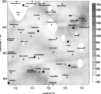
Fig. 1. Thirty-two German weather stations and eight forest climate stations (d) used in this study.
Distribution of 32 weather stations with complete ob-servational records for the period from 1965 to 1995, and eight forest climate stations with observed records (2–5 years) for the period 1991–1995 are shown in Fig. 1. An square root transformation was used for daily precipitation, because transforming daily precip-itation data in this way can reduce its skewness and/or improve precipitation prediction (Hutchinson et al., 1993; Kidson and Thompson, 1998).
2.2. Interpolation methods
2.2.1. Shepard method
In the Shepard (1968) method, interpolated values are computed from a weighted sum of the
observa-tions corrected by a locally computed increment. The details of calculation can be seen from Bussieres and Hogg (1989). A predetermined maximum radius (we used 100 km in this study) limits the number of the observational stations and the computed increment is based on local slopes as determined by a least-squares fit in orthogonal directions.
2.2.2. Closest station method
by a constant lapse rate (0.65◦C/100 m) for air temperatures.
2.2.3. Multiple linear regression (MLR)
A regional regression model was based on a first-degree polynomial (Russo et al., 1993):
Gi =a0+a1x+a2y+a3z (1)
where Gi is the estimated daily climatological vari-able, a the fit regression coefficients, x, y and z are
x-direction distance, y-direction distance and
eleva-tion, respectively.
2.2.4. Thin plate splines
TPS and kriging are formally equivalent but are formulated differently (Wahba, 1990; Hutchinson and Gessler, 1994). TPS are defined by minimising the roughness of the interpolated surface subject to the data having a predefined residual. Kriged surfaces are defined by minimising the variance of the error of esti-mation, which is normally dependent on a preliminary variogram analysis. TPS is usually accomplished auto-matically by choosing both the order of the derivative, which defines the surface roughness and the amount of data smoothing that is required to minimise the gen-eralised cross-validation. If there are n data values Gi at positions xi then it can be supposed that
Gi =f (xi)+εi (i=1,2, . . . , n) (2) where f (xi) is a function to be estimated from the observations Gi. Error termεi contains not only the measurement errors, but also purely local variability that is of much smaller scale than the resolution of any model to be fitted. xi are commonly co-ordinates in three-dimensional Euclidean space. Because TPS uses three-dimensional co-ordinates, it includes effect of environmental lapse rate (e.g., air temperature) on interpolated variables. Details can be found in Daley (1991) and Luo et al. (1998).
2.2.5. Barnes and Cressman method
BAR and CRE are distance weight interpolation methods. The computing details are given by Bussieres and Hogg (1989), and these two methods have been used for comparison of interpolation methods (Xia et al., 1999c) and reconstruction of monthly mean for-est climate data (Xia et al., 1999b).
2.3. Assessment criteria
As a test of the accuracy of each method, mean absolute error (MAE) and mean error (ME) are used as evaluation criteria (Hulme et al., 1995; Willmott and Matsuura, 1995). MAE provides a measure of how far the estimate can be in error, ignoring sign, and ME indicates the degree of bias.
2.4. Empirical transfer functions and examination of their stabilities
Wigley et al. (1990) used empirical transfer func-tions to obtain sub-grid-scale information from coarse-resolution general circulation model (GCM) output. They found that most of variance explained arises from the area average of air temperatures or precipitation which is the predictand: in other words, if the temperature, say, at a location is to be estimated, the best predictor is generally the area average tem-perature. Therefore, a univariate regression analysis (Kemp et al., 1983; Kim et al., 1984; Wigley et al., 1990) was used. It is defined as follows:
XF=a+bXW (3)
where a (offset) and b (slope) are the regression co-efficients, XF the measured climatological data at a site, and XWthe climatological data interpolated from the German weather stations to this site. These regres-sion equations were called empirical transfer func-tions. In order to eliminate the influence of seasonal variation on the accuracies of estimated forest climate data, daily forest climate data pooled over 4–5 years for each month were used. Therefore, 12 regression equations were established for each variable and for-est climate station.
variable and each forest climate station. We compared the change of correlation coefficients for the calibrated to independent data for each climatological element and each month. If the change is small, the regression equation is stable; otherwise, the equation is not sta-ble. Additionally, we will use the cross-validation to investigate the ME statistics in Section 3.2.1.
2.5. Reconstruction method
The reconstruction technique consists of two parts. First, we used TPS, as implemented in the ANUS-PLIN package (Hutchinson, 1997) to interpolate air temperatures at 32 weather stations to the six forest sites where forest climate stations were installed. TPS were chosen as a basic interpolation method, because we found that it can provide more accurate estimates for near-surface air temperatures and is appropriate for three-dimensional interpolation. Second, we used the empirical transfer functions to modify these interpo-lated air temperatures. These empirical transfer func-tions vary from month to month, from site to site and from meteorological variable to meteorological vari-able. Therefore, 216 empirical transfer functions were used in this study.
2.6. Quality control of reconstructed data
Because we used the empirical transfer functions to reconstruct long-term daily maximum temperature
Tmax, daily minimum temperature Tmin, and daily mean air temperature Tm, respectively, the relation-ship between Tmax, Tmin and Tm may not satisfy the requirement that Tmin < Tm < Tmax. If this case occurs, the quality of reconstructed air temperatures is questionable. Therefore, a final quality control is needed (Carlson et al., 1994; Meek and Hatfield, 1994; DeGaetano et al., 1995).
A very small percentage (<5%) of the reconstructed data values were flagged as erroneous in this study. In such cases, a manual adjustment was made for air tem-peratures. Usually, we assume the estimates of daily mean temperature are precise because of small MAE and the large explained variances for empirical trans-fer functions, then, we mainly adjust daily maximum temperature or daily minimum temperature. If Tmin (Tmax) is adjusted,Tmin(Tmax)= 2Tm−Tmax(Tmin). Finally, the adjusted daily forest climate data can be
used to calculate the temperature stress indices and to provide an input for the forest growth models.
3. Results and discussion
3.1. Comparisons of methods
3.1.1. Mean absolute error
Average results (averaged in time and spatially) of MAE between observed and estimated data at eight forest climate stations are summarised in Table 1. In general, MAE is smaller than 1.4◦C for daily maximum temperature and mean air temperature, is smaller than 0.9 hPa for daily water vapour pressure, and is smaller than 1.7◦C for daily minimum tem-perature for all six techniques. TPS yields the lowest MAE for all variables except for wind speed. SHE gives more accurate estimates for wind speed. Wind speed estimates using the SHE method are signif-icantly different from the other methods at the 5% level. Estimates of precipitation using TPS are signif-icantly different from the other methods (except for MLR) at the 5% level (t-test). For air temperatures and water vapour pressure, MLR estimates are as accurate as the TPS methods, but 15% of regression equations are not significant at the 5% level so that they cannot be used for daily minimum temperature. Therefore, MLR should be used with caution in this study area. According to this analysis, TPS is the more accurate interpolation technique for air temper-atures, water vapour pressure and precipitation, and SHE is the more accurate method for wind speed.
3.1.2. Temporal variation of mean absolute errors
We used TPS method (SHE method for wind speed) to interpolate the data of 32 German weather stations Table 1
Average results of MAE between observed and estimated values by six methods of Tmax, Tmin, Tm, e, u and P at eight forest
climate stations during the period 1991–1995
Variable BAR CRE CSM RRM SHE TPS
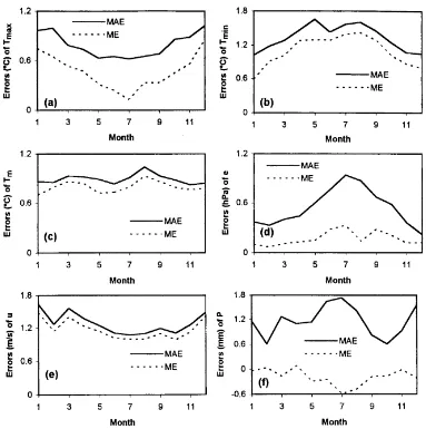
Fig. 2. Seasonal variation of MAE and ME between estimated and observed: (a) Tmax; (b) Tmin; (c) Tm; (d) e; (e) u; (f) P, averaged across
eight forest sites for the period 1991–1995.
to eight forest sites, and used observed forest climate data to calculate MAE and ME for the period from 1991 to 1995. The averaged results of eight forest cli-mate stations are shown in Fig. 2. For daily maximum temperature, MAE is largest in winter and smallest in summer, ranging from 1.0◦C in December to 0.6◦C in July (Fig. 2a), however, for daily minimum tempera-ture, MAE is smallest in winter and largest in sum-mer, ranging from 1.7◦C in May to 1.0◦C in January (Fig. 2b). For daily mean temperature, seasonal varia-tion of MAE is smaller, and MAE ranges from 1.0◦C in August to 0.8◦C in November (Fig. 2c). MAE of
1.7 mm in July to 0.6 mm in February and October (Fig. 2f).
ME are positive for all variables except precipita-tion. This means that the TPS method overestimates daily maximum temperature, minimum temperature, mean air temperature and water vapour pressure and underestimates daily precipitation; the SHE method overestimates daily wind speed (Fig. 2). This overes-timate may be due to forest effect of daily maximum, minimum, mean temperature and wind speed, because the air temperatures (wind speed) within forests are lower (smaller) than outside of forests.
3.1.3. Spatial variation of mean absolute errors
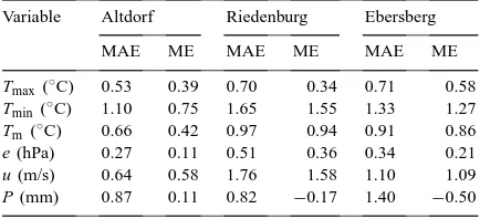
Usually, the spatial distribution of MAE of mete-orological variables is determined by elevation, land surface covering, slope inclination, slope orientation and the density of the station network (i.e., Bussieres and Hogg, 1989). We used MLR to study the rela-tionship between MAE and these physical factors. As we have only eight forest climate stations, none of the regression equations were significant at the 5% level for all variables. We selected three forest cli-mate stations, station Altdorf (located in a plain area), station Riedenburg (located in a valley), and station Ebersberg (foothills of the Alps). MAE and ME of variables at these stations are listed in Table 2. For daily air temperatures, MAE are larger at the valley and hill stations than at the plain station because of topographic effects, although TPS considers the influ-ence of lapse rates. For water vapour pressure, MAE is larger at the valley station than at the plain station and the hill station. For wind speed, MAE is largest at the valley station. For precipitation, MAE is much
Table 2
MAE and ME for Tmax, Tmin, Tm, e, u and P at three forest
climate stations for the period 1991–1995
Variable Altdorf Riedenburg Ebersberg
larger at hill station than at valley and plain stations. The results are similar for ME.
3.1.4. Meteorological stress factors
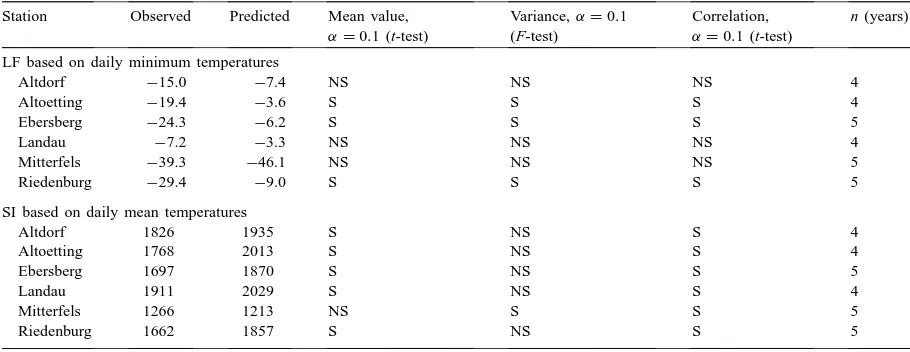
The purpose of estimating forest climatological data is for use in forest studies (i.e., forest damage), therefore, the accuracy of the predicted meteorologi-cal stress factors (see Appendix A) must be discussed. We used the TPS method to interpolate the data from 32 German weather stations to the six forest sites (we exclude Freising and Schongau stations because of short observational records), and then used these interpolated data and observed data to calculate the meteorological stress factors. The results from the statistical examination are listed in Table 3.
Predicted and observed heat and winter indices are not significantly different at the 10% level for all six examined stations, even though the predicted heat and winter indices are warmer than observed ones. This is consistent with previous comparisons (Fig. 2) where predicted daily air temperatures are higher than the observed station temperatures.
Table 3
Observed and predicted LF (◦C days) and SI (◦C days) based on observed daily minimum and mean temperatures, respectively, and the
data sets which are interpolated by using TPS at six forest climate stations Station Observed Predicted Mean value,
α=0.1 (t-test)
LF based on daily minimum temperatures
Altdorf −15.0 −7.4 NS NS NS 4
SI based on daily mean temperatures
Altdorf 1826 1935 S NS S 4
Altoetting 1768 2013 S NS S 4
Ebersberg 1697 1870 S NS S 5
Landau 1911 2029 S NS S 4
Mitterfels 1266 1213 NS S S 5
Riedenburg 1662 1857 S NS S 5
et al. (1998). Their predicted and observed phenolo-gies and whole canopy respirations were significantly different at four of the five stations. Although MAE between predicted and observed air temperatures are much smaller in our study (<1.7◦C) than those in their study (<3.0◦C), some estimated stress factors can still not be used.
Therefore, more accurate estimated forest climate data are needed for calculating various meteorological stress factors (i.e., LF). Empirical transfer functions may be an appropriate method, because they show large improvement for monthly mean forest climato-logical data (Xia et al., 1999b).
3.2. Empirical transfer function development
We develop simultaneous relationships between the interpolated data (i.e., the predictors) and observed forest climate data (i.e., the predictands) for a partic-ular forest site. We use a univariate regression to de-velop separate functions for each predictand and each month. These functions can implicitly incorporate the effects of land cover (i.e., forest), local topography and geography.
3.2.1. Explained variance
The strongest statistical relationships between the predictands and predictors is for daily maximum tem-perature, mean air temperature and water vapour
pres-sure at the eight Bavarian forest climate stations, as indicated by the large explained variances. Normally, the explained variances are larger than 0.90 for most of eight forest sites. For daily minimum temperature, the statistical relationship between observed values and interpolated values is also strong, usually the ex-plained variances are larger than 0.88 for all eight forest climate stations. The statistical relationship be-tween observed and interpolated for precipitation and wind speed is weak (explained variance is smaller than 0.8 except precipitation at two sites).
Since a major problem evident in the previous sec-tions is MAE and ME, the cross-validation process described in Section 2.4 was used to investigate both these errors. The examination results of independent samples (year 1995) show that the transfer functions greatly reduce MAE and ME for all climate variables except for precipitation, particularly minimum air tem-perature, mean air temperature and wind speed at the five examined stations (Altdorf, Altoetting, Ebersberg, Landau, Riedenburg).
3.2.2. Regression equations (transfer functions)
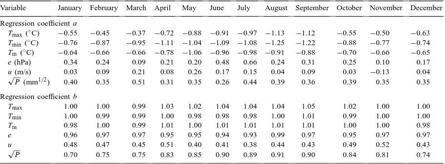
Table 4
Regression coefficients a and b averaged across eight sites for Tmax, Tmin, Tm, e, u and P
Variable January February March April May June July August September October November December Regression coefficient a
represent the forest influence on daily minimum tem-perature and mean air temtem-perature. The effect is−1.3 to−0.9◦C in summer and−0.8 to−0.6◦C in winter. For wind speed, a is not significantly different from zero at the 5% level. It is clearly shown that forest reduces wind speed by 49–62% at eight forest sites (Table 4). For daily maximum temperature, the forest effect is smaller than 0.8◦C when we consider role of
a and b for the summer (offset is also negative but
slope is significantly different from unity). Thus, these effects can be included by the a and/or b of the em-pirical transfer functions. For water vapour pressure and precipitation, the offset and slope include the for-est effect as well. These results are based on the av-erage of eight forest sites. In practice the forest effect on daily air temperatures, water vapour pressure and wind speeds varies from site to site.
3.2.3. Importance, temporal stability and spatial availability of empirical transfer functions
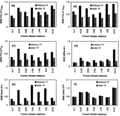
A summary of the errors obtained from seven forest climate stations is presented in Fig. 3. The empirical transfer functions greatly reduce the errors between observed and estimated values for all meteorological variables except daily precipitation. When empirical transfer functions were used, MAE were reduced by 40–90% for daily wind speed depending on the dif-ferent forest climate stations (Fig. 3e), 20–60% for daily minimum temperature (Fig. 3b), 30–70% for daily mean temperature (Fig. 3c), and less than 40%
for daily maximum temperature and water vapour pressure for all forest climate stations except for for-est climate station Schongau (Fig. 3a and d). The improvements of empirical transfer functions vary from site to site, and from variable to variable. But for daily precipitation, MAE were hardly reduced (Fig. 3f) by the use of empirical transfer functions.
The analysis shows that the empirical transfer func-tions are important for estimating daily minimum tem-perature, mean air temperature and wind speed. They also improve the estimates of daily maximum tem-perature and water vapour pressure, although the im-provement is not significant. However, they cannot improve the estimates of daily precipitation. In addi-tion, the empirical transfer functions can also hardly improve the estimates of all six variables at Mitterfels mountain forest climate station.
Fig. 3. MAE between observed and estimated: (a) Tmax; (b) Tmin; (c) Tm; (d) e; (e) u; (f) P at seven sites (TF: transfer function; Alt:
Altdorf; AOE: Altoetting; EBE: Ebersberg; FRE: Freising; LAN: Landau; RIE: Riedenburg; SOG: Schongau).
mean values is smaller than 11% for LF at all five sta-tions. There is almost no difference between observed and estimated mean SI for all five stations.
The differences between observed and estimated mean heat and winter indices become smaller, when the empirical transfer functions were used. Thus, the empirical transfer functions improve the estimation ac-curacies for the mean heat and winter indices at five stations, even though the improvement is not as large as that for LF and SI.
Table 5
Observed and estimated late frosts and SI based on observed daily minimum temperatures and mean temperatures, respectively, and the data sets which are estimated by using empirical transfer functions for five sites
Station Observed Estimated Mean value, α=0.10 (t-test)
Variance,α=0.10 (F-test)
Correlation, α=0.10 (t-test)
n (years)
LF based on daily minimum temperatures
Altdorf −15.0 −15.0 NS NS S 4
Altoetting −19.4 −17.9 NS NS S 4
Ebersberg −24.3 −21.7 NS NS S 5
Landau −7.2 −7.8 NS NS S 4
Riedenburg −29.4 −26.2 NS NS S 5
SI based on daily mean temperatures
Altdorf 1862 1860 NS NS S 4
Altoetting 1768 1767 NS NS S 4
Ebersberg 1697 1698 NS NS S 5
Landau 1911 1912 NS NS S 4
Riedenburg 1662 1661 NS NS S 5
pressure, the empirical transfer functions are stable, but for daily wind speed, empirical transfer functions are not stable (not shown). In addition, we discussed the spatial applicability of empirical transfer func-tions. We used the observed data and interpolated data (Ebersberg station) to establish empirical trans-fer functions, and then we used these functions and interpolated data (Altoetting station, 80 km distant with the similar topography and same species) to estimate climate data and calculate MAE and ME. The results show large errors for all six variables at Altoetting station. It means that, these empirical trans-fer functions, established in a forest region, cannot be
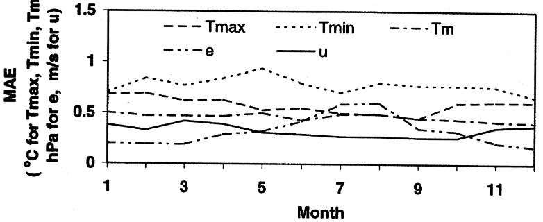
Fig. 4. Seasonal variation of MAE averaged across seven sites for Tmax, Tmin, Tm, e and u when the empirical transfer functions were used.
3.2.4. Accuracy of estimated data
The MAE averaged across seven stations (except for Mitterfels station) are shown in Fig. 4. Usually, the estimated errors ranged from 0.49◦C in September to 0.69◦C in February for daily maximum temperature, ranged from 0.66◦C in December to 0.94◦C in May for daily minimum temperature, and ranged from 0.41◦C in December to 0.5◦C in May for mean temperature (Fig. 4). Errors less than 1◦C can thus be expected for air temperatures. Errors ranged from 0.17 hPa in December to 0.6 hPa in August for water vapour, and for wind speed ranged from 0.26 m/s in September to 0.40 m/s in April (Fig. 4). These estimated forest cli-mate data are relatively accurate, when we compared the estimates of climatological data without the em-pirical transfer functions.
Of the seven forest sites, the low elevation site (e.g., Landau) has smaller errors while the high elevation site (e.g., Schongau) has larger errors. For daily mini-mum temperature, the forest site Riedenburg has large errors because of its location in a valley.
3.3. Reconstruction and application of 31-year forest climate data
3.3.1. Temporal and spatial variation of near-surface air temperature
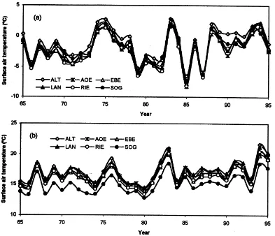
Firstly, we used the method described in Section 2.5 to reconstruct 31-year forest climate data at six of the eight forest sites except for Freising and Mitterfels sta-tions. Secondly, we use the quality method presented in Section 2.6 to correct the erroneous data. The re-constructed near-surface air temperatures in January and July (averages of all days for these 2 months) are presented in Fig. 5. The temporal variations of air tem-peratures at six forest climate stations are relatively consistent, although there are differences among the stations. The coldest years are 1979, 1985 and 1987 (Fig. 5a), and the warmest years are 1976, 1983, 1991 and 1994 (Fig. 5b). Near-surface air temperatures are different at six forest sites. The differences between stations are not large in January, but it is very large in July. Generally speaking, low elevation sites have higher near-surface air temperatures (e.g., Altdorf) and high elevation sites have lower near-surface air tem-peratures (e.g., Schongau). The largest difference may be up to 3◦C.
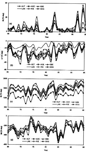
3.3.2. Temporal and spatial variation of stress indices
3.3.2.1. Heat index. HI (see Appendix A) describes
the possible effect of high temperatures on forest trees. The calculated HI at the six forest sites is shown in Fig. 6a. The largest index occurred in 1976, 1983, 1992 and 1994. These years are warmest when the variation of near-surface air temperatures is analysed at the six forest sites (Fig. 5a). This means that HI is closely relating to the anomalies of the regional climates.
The heat indices at the six forest sites are very dif-ferent from each other (Fig. 6a). Heat indices at forest sites Ebersberg and Schongau are much smaller than those at the other four sites for the anomaly year 1976, 1983 and 1994. Thus, high temperatures may not dam-age the forest trees at these two forest sites, because they are located on the high elevation ridges (station Ebersberg: 540 m, station Schongau: 780 m), and max-imum temperatures are lower at the two sites than the other four sites. Clearly, local climates greatly modify the heat indices at the two sites. Therefore, the inter-actions between regional (global) climate anomalies and local environments may greatly affect local heat indices, but regional climate anomalies influence the whole study area and local environments affect only a specific forest site.
3.3.2.2. Late frost. LF (see Appendix A) describes
the average intensity of LF damage to trees. It is pre-sented in Fig. 6b for the six forest sites. The strongest LF occurred in 1973, 1982 and 1984, with relatively strong LF also occurring in 1977 and 1992. The LF is very different at six forest sites, it varies from site to site, and from year to year (Fig. 6). The Landau site experiences fewer LF because of its low elevation, and Schongau site located on a high elevation ridge and Riedenburg site located in the valley experience more frequent LF because of the high elevation and valley topography. Valley floors will often be colder than ridge sites because cold air drainage and radia-tion cooling will lead to a temperature inversion.
Fig. 5. Near-surface air temperatures at six forest sites for: (a) January; (b) July (ALT: Altdorf; AOE: Altoetting; EBE: Ebersberg; LAN: Landau; RIE: Riedenburg; SOG: Schongau).
different at each of the six forest sites. Low elevation sites have the larger SI (e.g., Altdorf, Landau) and high elevation sites have the smaller SI (e.g., Schongau).
3.3.2.4. Winter index. Winter index (WI) can be
used to represent the severity of the winter. The cold-est years were 1969, 1985 and 1987. The warmcold-est year was 1974. WI also shows the difference be-tween sites. This difference varies from year to year (Fig. 6d). Spatial variation of WI is similar to that of SI, but the difference between two sites is much smaller.
We compared the 31-year averaged values of four meteorological stress factors estimated with and with-out the empirical transfer functions. The averaged
dif-ference of the estimated index is 15% for SI and HI, 20% for WI and 40% for LF at six forest sites. These differences are not negligible because they are signifi-cant at the 5% level. Therefore, the use of air temper-atures directly interpolated from weather stations may result in the inaccurate estimates of derived variables (e.g., LF).
3.3.3. Uncertainties of meteorological stress factors
or more) for an individual year. The second source of uncertainty is a physiological one. Based on our knowledge, threshold values were chosen for the tem-perature stress indices: 0◦C for the WI, 5◦C for the SI, and 30◦C for the HI. Effects of chosen threshold val-ues on the relationships with defoliation are unknown. Furthermore, no difference was made between sensi-tivity for particular tree species, which also introduced some uncertainty, since the threshold values vary from tree species to tree species. In addition, it should be noted that these forest climate data measured in a for-est clearing can introduce the large uncertainties, be-cause they are not measured within a forest canopy or above a forest canopy.
Besides the four meteorological factors, we used daily mean temperatures to calculate growing-degree days, which is important for agriculture and forestry. In USA, the mean value of daily maximum and mini-mum temperature was used for daily mean temperature (McMaster and Wilhelm, 1997), although the mean temperatures calculated using hourly temperatures can improve the accuracy of predictions (Cross and Zuber, 1972). Because we have 15 min observational records at six forest sites, we compare daily mean temperature calculated by 15 min records to mean temperature cal-culated according to three standard observation times (7:30, 14:30, and 21:30 h) of German Weather Service, and average of daily maximum and minimum tem-peratures at six forest sites for the period from 1991 to 1995. We found that the difference between daily mean values according to 15 min records and three standard observational times is small. We determine to use daily mean temperature calculated by three stan-dard observational times, because we believe that the value is more close to true daily mean temperature.
4. Conclusions
We observed significant differences in the accuracy of the BAR, CRE, CSM, MLR, SHE and TPS for pre-diction of the six climate variables. In general, TPS can give more accurate estimates of daily maximum tem-perature, minimum temtem-perature, air temtem-perature, wa-ter vapour pressure and precipitation, while the SHE is more accurate method for wind speed.
We developed the empirical transfer functions be-tween observed and interpolated data using a
univari-ate regression technique and examined their effects for all forest sites. The results show that empirical transfer functions improve the estimates of air temperatures, water vapour and wind speed for seven of the eight forest sites, particularly wind speed, daily minimum and mean temperature, since they include forest im-pacts on daily climatological data, as described in this paper. However, they cannot improve the estimate of daily precipitation for any forest site. The examination of LF and SI shows that the observed and estimated values are consistent for five forest sites, whereas, they are significantly different at the 10% level when em-pirical transfer functions are not used. Therefore, the empirical transfer functions are essential to estimate reliable climatological data for the forest sites.
Acknowledgements
We would like to express our thanks to colleagues of German Weather Service and Bavarian State Insti-tute of Forestry for their timely provision of climate data. Normand Bussieres and Mike Hutchinson kindly provide the interpolation software. We wish to thank Dr. J.B. Stewart and two anonymous referees whose comments greatly improved the quality of this paper.
Appendix A. Calculation of the meteorological stress factors
In order to compare the accuracy of estimated climatological data, we define four stress indices (Hendriks et al., 1997):
1. Winter index (WI): it indicates the severity of the winter. This index equals the sum of daily mean temperature below 0◦C in the period from 1 November to 31 March (unit: degree days). 2. Late frost (LF): late-night frost in spring may
cause serious damage to trees when growth has just started and, buds and young shoots are very sensitive to frost. This parameter is defined as the sum of minimum temperature (below 0◦C) in the period from 1 April to 30 June.
value of 30◦C which is used in Bavarian Climate Atlas (BayForKlim, 1996).
4. Summer index (SI): this quality of the growing sea-son is included, since it influences the potential photosynthetic activity and the ability to the tree to produce reserve assimilates for the purposes of defence and growth in the beginning of the next season. This factor is sum of the differences be-tween daily mean temperatures during the growing season and a threshold value of 5◦C.
References
Barnes, S.L., 1973. Mesoscale objective map analysis using weighting time-series observations. NOAA Tech. Memo. ERL NSSL-62. US Department of Commerce, 60 pp.
BayForKlim, 1996. Klimaatlas von Bayern. Kanzler, München, Germany.
Bolstad, P.V., Swift, L., Collins, F., Regniere, J., 1998. Measured and predicted temperatures at basin to regional scales in the southern Appalachian mountains. Agric. For. Meteorol. 91, 161–176.
Bussieres, N., Hogg, W., 1989. The objective analysis of daily rainfall by distance weighting schemes on a mesoscale grid. Atmos. Ocean 27, 521–541.
Carlson, R.E., Enz, J.W., Baker, D.G., 1994. Quality and variability of long-term climate data relative to agriculture. Agric. For. Meteorol. 69, 61–74.
Cressie, N.A.C., 1985. Fitting variogram models by weighted least-squares. Math. Geol. 17, 563–586.
Cressman, G.P., 1959. An operational objective analysis system. Monthly Weather Rev. 87, 367–374.
Cross, H.Z., Zuber, M.S., 1972. Prediction of flowering dates in maize based on different methods of estimating thermal units. Agron. J. 64, 351–355.
Daley, R., 1991. Atmospheric Data Analysis. Cambridge University Press, London, 457 pp.
DeGaetano, A.T., Eggleston, K.L., Knapp, W.W., 1995. A method to estimate missing maximum and minimum temperature observations. J. Appl. Meteorol. 34, 371–380.
Dodson, R., Marks, D., 1997. Daily air temperature interpolated at high spatial resolution over a large mountainous region. Climate Res. 8 (1), 1–20.
Hendriks, K., Klap, J., Je Joung, E., Van Leeuwen, E., De Vries, W., 1997. Calculation of natural stress factors. In: Ten Years of Monitoring Forest Condition in Europe. EC-UN/ECE, Brussels, Geneva, pp. 225–240.
Hewitson, B., 1994. Regional climates in the GISS general circulation model: air surface temperature. J. Climate 7, 283– 303.
Hewitson, B., Crane, R.G., 1992a. Regional climates in the GISS global circulation model: synoptic-scale circulation. J. Climate 5, 1001–1002.
Hewitson, B., Crane, R.G., 1992b. Regional-scale climate prediction from the GISS GCM. Palaeogeogr. Palaeoclimatol. Palaeoecol. 97, 249–267.
Hulme, M., New, M., 1997. Dependence of large-scale precipitation climatologies on temporal and spatial sampling. J. Climate 10, 1099–1113.
Hulme, M., Conway, D., Jones, P.D., Jiang, T., Barrow, E.M., Turney, C., 1995. Construction of a 1961–1990 European climatology for climate change modelling and impact applications. Int. J. Climatol. 15, 1333–1363.
Hutchinson, M.F., 1997. ANUSPLIN, Version 3.2. World Wide Web. http://cres.anu.edu.au/software/anusplin.html.
Hutchinson, M.F., 1998. Interpolation of rainfall data with thin plate smoothing splines. I. Two-dimensional smoothing of data with short range correlation. J. Geogr. Inform. Decision Anal. 2, 153–167.
Hutchinson, M.F., Gessler, P.E., 1994. Splines more than just a smooth interpolator. Geoderma 62, 45–67.
Hutchinson, M.F., Richardson, C.W., Dyke, P.T., 1993. Normalisation of rainfall across different time steps. In: Management of Irrigation and Drainage Systems, July 21–23, 1993, Park City, UT. Irrigation and Drainage Division, ASCE, US Department of Agriculture, pp. 432–439.
Huth, R., Nemesova, I., 1995. Estimation of missing daily temperature: can a weather categorisation improve its accuracy? J. Climate 34, 1901–1916.
Karl, T.R., Wang, W.C., Schlesinger, M.E., Knight, R.W., 1990. A method of relating general circulation model simulated climate to the observed local climate. Part I: Seasonal statistics. J. Climate 3, 1053–1079.
Kemp, W.P., Burnell, D.G., Everson, D.O., Thomson, A.J., 1983. Estimating missing daily maximum and minimum temperatures. J. Climate Appl. Meteorol. 22, 1587–1593.
Kidson, J.W., Thompson, C.S., 1998. A comparison of statistical and model-based downscaling techniques for estimating local climate variations. J. Climate 11, 735–753.
Kim, J.W., Chang, J.T., Baker, N.L., Wilks, D.S., Gates, W.L., 1984. The statistical problem of climate inversion: determination of the relationship between local and large-scale climate. Monthly Weather Rev. 112, 2069–2077.
Kunkel, K.E., 1989. Simple procedures for extrapolation of humidity variables in the mountainous western United States. J. Climate 2, 656–669.
Luo, Z., Wahba, G., Johnson, D.R., 1998. Spatial–temporal analysis of temperature using smoothing spline ANOVA. J. Climate 11, 18–28.
Meek, D.W., Hatfield, J.L., 1994. Data quality checking for single station meteorological databases. Agric. For. Meteorol. 69, 85– 109.
McMaster, G.S., Wilhelm, W.W., 1997. Growing degree-days: one equation, two interpretations. Agric. For. Meteorol. 87, 291– 300.
Mueller-Edzards, C., Vries, W.D., Erisman, J.W., 1997. Ten Years of Monitoring Forest Condition in Europe. EC-UN/ECE, Brussels, Geneva, 386 pp.
Preuhsler, T., Adler J., Dreier, P., 1996. Bayerische Waldklimastationen Jahrbuch 1995. Bayerische Landesanstalt für Wald und Forstwirtschaft, Sachgebiet Forsthydrologie. Freising, Germany, 110 pp.
Running, S., Nemani, R., Hungerford, R., 1987. Extrapolation of synoptic meteorological data in mountainous terrain and its use for simulating forest evapotranspiration and photosynthesis. Can. J. For. Res. 17, 472–483.
Russo, J.M., Liebhold, A.M., Kelley, J.G.W., 1993. Mesoscale weather data as input to a gypsy moth (Lepidoptera: Lyman-triidae) phenology model. J. Econ. Entomol. 86, 838–844. Shepard, D., 1968. A two-dimensional interpolation function for
irregularly spaced data. In: Proceedings of the 1968 ACM National Conference, pp. 517–524.
Wahba, G., 1990. Spline models for observational data. CBMS–NSF Regional Conference Series in Applied Mathe-matics, 169 pp.
Wallis, J.R., LettenMayer, D.P., Wood, E.F., 1991. A daily hydroclimatological data set for the continental United States. Water Resourc. Res. 27, 1657–1663.
Wigley, T.M.L., Jones, P.J., Briffa, K.R., Smith, G., 1990. Obtaining sub-grid-scale information from coarse-resolution
general circulation model output. J. Geophys. Res. 95, 1943– 1953.
Willmott, C.J., Matsuura, K., 1995. Smart interpolation of annually averaged air temperature in the United States. J. Appl. Meteorol. 34, 2577–2586.
Winkler, J.A., Palutikof, J.P., Andresen, J.A., Goodess, C.M., 1997. The simulation of daily temperature time series from GCM output. Part II: Sensitivity analysis of an empirical transfer function methodology. J. Climate 10, 2514–2532.
Xia, Y., 1999. Empirical transfer functions — applications for estimation and reconstruction of meteorological data at Bavarian forest climate stations. Dissertation. The University of Munich, Germany.
Xia, Y., Fabian, P., Stohl, A., Winterhalter, M., 1999a. Forest climatology: estimation of missing values for Bavaria, Germany. Agric. For. Meteorol. 96, 131–144.
Xia, Y., Fabian, P., Stohl, A., Winterhaler, M., 1999b. Forest climatology: reconstruction of mean climatological data for Bavaria, Germany. Agric. For. Meteorol. 96, 117–129. Xia, Y., Winterhalter, M., Fabian, P., 1999c. A model to interpolate