MERGING DIGITAL SURFACE MODELS IMPLEMENTING BAYESIAN APPROACHES
H. Sadeq a,*,J. Drummond b, Z. Li c
a Surveying Eng. Dep., College of Engineering, Salahaddin University-Erbil, Kirkuk Road, Erbil-Iraq- [email protected] b School of Geographical and Earth Sciences, University of Glasgow, Glasgow G12 8QQ, UK
c School of Civil Engineering and Geosciences, Newcastle University, Newcastle upon Tyne, NE1 7RU, UK
Commission VII, WG VII/6
KEY WORDS: Bayesian approaches, Likelihood, local entropy, Merging DSMs, WorldView-1, Pleiades
ABSTRACT:
In this research different DSMs from different sources have been merged. The merging is based on a probabilistic model using a Bayesian Approach. The implemented data have been sourced from very high resolution satellite imagery sensors (e.g. WorldView-1 and Pleiades). It is deemed preferable to use a Bayesian Approach when the data obtained from the sensors are limited and it is difficult to obtain many measurements or it would be very costly, thus the problem of the lack of data can be solved by introducing a priori estimations of data. To infer the prior data, it is assumed that the roofs of the buildings are specified as smooth, and for that purpose local entropy has been implemented. In addition to the a priori estimations, GNSS RTK measurements have been collected in the field which are used as check points to assess the quality of the DSMs and to validate the merging result. The model has been applied in the West-End of Glasgow containing different kinds of buildings, such as flat roofed and hipped roofed buildings. Both quantitative and qualitative methods have been employed to validate the merged DSM. The validation results have shown that the model was successfully able to improve the quality of the DSMs and improving some characteristics such as the roof surfaces, which consequently led to better representations. In addition to that, the developed model has been compared with the well established Maximum Likelihood model and showed similar quantitative statistical results and better qualitative results. Although the proposed model has been applied on DSMs that were derived from satellite imagery, it can be applied to any other sourced DSMs.
1. INTRODUCTION
DSMs performs an important role in various applications such as: planning; 3D urban city maps; natural disaster management (e.g. flooding, earthquake, landslide); civilian emergencies; military activities; airport management; and, geographical analysis, such as crime and hazards (Saeedi and Zwick 2008). Due to an increase in the sources of DSMs, their generation has led to a focus on merging datasets to produces a single one incorporating the data from multiple sources. Different terms have been used to indicate the merging such as fusion, combination, integration and synergy. These all can be considered to be a synonym for merging (Papasaika-Hanusch, 2012).
Data merging has been studied by different researchers. For instance, it can be used, potentially, to identify the highest quality data for an area, as well as to address problems of data volume. Data merging is also important as it fills the gaps and voids produced while constructing the original DEMs. The obvious solution for merging DEMs is to average tiles or strips from DEMs of the same area, and to produce a seamless DSM (Reuter, Strobl and Mehl, 2011), but this will not reflect the original data quality, because it gives the same weight to all data.
Data merging has been shown to be important for increasing data quality Podobnikar (2007), Lee et al. (2005), Fuss (2013), Papasaika et al. (2009), and Dowman (2004). Wegmüller et al. (2010), focussed on the value of DSM merging to fill gaps. Hosford et al. (2003) showed an approach for enhancing DSMs through a merging operation based on a geostatistical approach (i.e. one capable of estimating a σ value).
Papasaika et al. (2009) used merging to solve the problem of poor image matching technique by incorporating extra data sources.
Schultz et al. (1999) used merging for image mosaicking using different data sources (SRTM SAR-X, ERS SAR tandem data).
The purpose of this research was to increase DSM accuracy, based on an area’s morphological characteristics. Two pairs of satellite images have been used in this research, first the DSMs have been produced, and later they have been merged using both Maximum Likelihood and Bayesian approaches. Later the results have been evaluated by using check points measured in the field.
The approach that has been suggested in this research is based on Bayes rule which requires incorporation of a priori data. The result has been compared with those achieved using the Maximum Likelihood approach. This account is structured to discuss: Bayesian inference in section 2; the test site in section 3; ; the DSM formation model is in section 4; methodology in section 5; results and analyses in section 6; and, finally, the conclusion is given in section 06.
2. BAYESIAN INFERENCE
for the unobserved data through a process called Bayesian inference. The values used in Bayesian approaches are random variables and provide uncertainties as output, represented as probability expressions. Bayesian inference encompass statistical inference methods where observations are utilized to determine the probability that assumptions are likely to be true, or to revise an already determined probability. In the applied field, Bayesian inference uses a priori probability calculated from the likelihood of certain assumptions regarding the observations imported into a computation or process.
Bayesian inference can be summarized as using a model which is constructed based on Bayes’ Rule, and the obtained data represented by a probability form which is called the a posteriori probability distribution. The model used in Bayesian inference should effectively reflect the condition from which information is to be inferred. Bayesian inference is represented by constructing a model that adequately represents the situation from which information is to be inferred. The constructed model
is based on Bayes’ Rule in which the results are represented by probability and called the a posteriori probability distribution. The elements used in Bayesian inference are based on the likelihood and a priori probability. The likelihood is arises by fitting a probability to the data in the experiment, while the a priori probability refers to subjective belief about the situation before that data gathering (Gelman et al., 2004). The major features of Bayesian inference that have led it to becoming a focus for researchers can be specified as: using the probability of the parameters to measure uncertainty instantaneously; handling any number of parameters; and, the applicability of joint probability density functions (Gelman et al., 2004).
According to the literature, Bayesian approaches have been applied in remote sensing, successfully, to fuse and segment images (Mascarenhas, Banon and Candeias, 1992; Zaniboni and Mascarenhas, 1998; Punska, 1999; Mohammad-Djafari, 2003; Shi and Manduchi, 2003; Feron and Mohammad-Djafari, 2004; Ge, Wang and Zhang, 2007; Gheta, Heizmann and Beyerer, 2008; Zhang, 2010) but no study has been found relating to their use in merging or fusing digital surface models. The common approach to fusing DSMs is based on using a weighted average,
after assigning weights to the DSMs’ points based on checking their fidelity or performing a “DSM accuracy assessment” by
calculating some statistical measurements (i.e. RMSE).
3. TEST SITE
For the test, two sources of satellite images have been acquired with the specifications as shown in the Table 1 (the first source was from the Worldview-1 (WV-1) sensor from the Digital Globe organization). As shown in Table 1the time gap between the satellite imagery is calculated to be around 14 months. However it has been assumed, in this research, that no changes have arisen within the time period, therefore the merging in this research does not consider any multitemporal effect. This assumption has been made in order to focus on the effect of the merging using a Bayesian approach.
Image ID Acquisition
Date Image Type Pan/MS Band GSD(m) Res. WV-1 image1 24/05/2012
11:42:49.42
Panchromatic 1/- 0.5
WV-1 image2 24/05/2012 11:43:28.78
Panchromatic 1/- 0.5
Pleiades image1 09/07/2013 11:35:44.1
Pansharpened 1/4 0.5
Pleiades image2 09/07/2013 11:36:25.8
Pansharpened 1/4 0.5
Table 1. Characteristics of the used satellite imageries
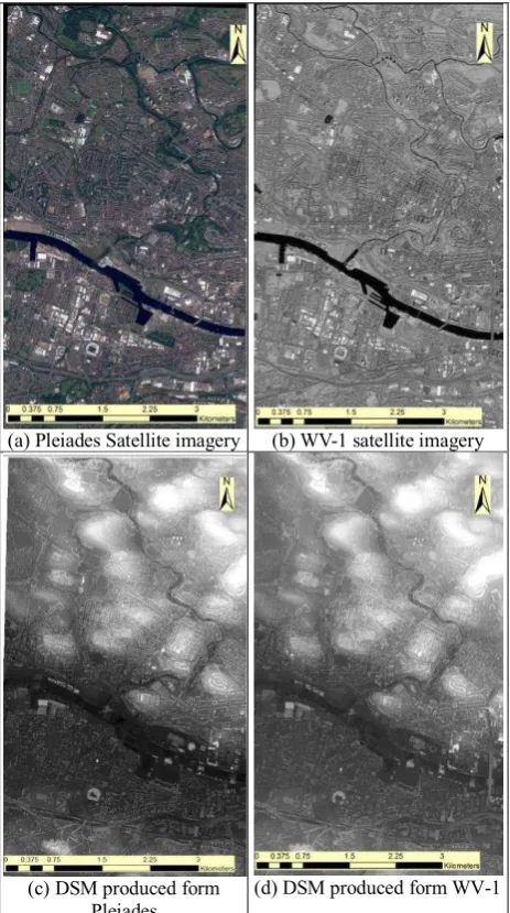
The test area used to merge the DSMs is located in Glasgow, United Kingdom, covering 10km2, Figure 1. The test area coordinates were on the Universal Transverse Mercator (UTM)
projection, longitudinal zone 30 ‘North’ using the WGS84 figure
of the Earth for both the vertical and horizontal datum. The area had coordinates, bottom left corner (417820 mE, 6191335 mN) and upper right (420527 mE, 6195090 mN).
The data have been processed and rectified for DSM production using Socet GXP 4.1 software, with the aid of GCPs. Using SOCET-GXP, the resolution of the DSMs was 1m. It is recommend by the SOCET GXP provider that the orthoimagery resolution be higher than the GSD of the DSM (Zhang and Smith, 2010).
(a) Pleiades Satellite imagery (b) WV-1 satellite imagery
(c) DSM produced form
Pleiades (d) DSM produced form WV-1
Figure 1. Study area and study data used in merging DSMs
4. DSM FORMATION AND MERGING MODEL
The blunders and systematic errors can be handled, but for the random errors this is not possible. Therefore the underlying DSM contained errors embedded in it. Equation 1, which can also be referred to as the forward model, is used to relate the true DSM, referred to as DSM̅̅̅̅̅̅̅, to that obtained from satellite imagery technique (DSM)
:
Z , = Z̅ , + ε , (1)
Where: Z is the generated height of the DSM at location x,y,
Z
̅
is the elevation of true underlying DSM̅̅̅̅̅
at location x,y, and,ε is the height error in each DSM at location x,y.
Merging DSMs can be considered as an ill-posed problem. According to Hadamard (1902), cited via Beyerer et al.(2011) a problem is considered to be ill-posed in the following cases: if a solution is not unique; the problem does not have solution; or, the result can become significantly different following a small change in the input data.
Due to the intrinsic random error in the DSM, the result obtained from the merging is not unique and therefore the merging problem is considered an ill-posed problem. The processing model used arises from considering the combination of the actual digital surface model values, represented by DSM
̅̅̅̅̅
, and noise, through a simple transformation from the measured noisy digital surface model, represented by DSM, to the DSM̅̅̅̅̅
, at each point in the model. The model for generating the data, developed from equation 1, is shown in equation 2,(
In order to obtain the required DSM the above model is used to form the inverse model.
The measured DSMs are referred to as DSM1 to DSMk, while the underlying real or latent DSM values are represented by DSM
̅̅̅̅̅
and the errors at each location in the DSM are represented by Maximum Likelihood (the weighted average approaches) and Bayesian approaches are discussed in this section. For both approaches, first quality assessment has been performed to find the accuracy of each DSM. Then later the Maximum Likelihood merging was executed. Regarding the Bayesian merging in addition to the quality assessment the a priori estimation is determined in the probability form.5.1 Digital Surface Model (DSM) Quality Assessment
To start the merging process it is necessary to find out the quality of each digital surface model. DSM quality is an intensely researched topic commencing about 40 years ago, in 1972, led by Makarovic (Li, 1990), in The Netherlands. The quality of the DSM is based on measuring the error in DSM heights.
There are many factors affecting the accuracy of a DSM, according to Chen and Yue (2010), Li (1992) and Papasaika-Hanusch (2012), such as:
distortion inherent in the sensor;
the source data’s attributes such as density and spread; surface or terrain features such as relief, land-cover, and
texture;
the mathematical approach that has been implemented to produce the DSM from the data source or the interpolation methods used; and,
techniques used in map-digitization or field surveying.
The quality index that has been used foremost in this study to represent the quality of DSMs is a single RMSE value per terrain model, equation 3, based on using the measured ground control points. In addition to assuming the errors are distributed uniformly, it has been assumed the images are fully registered; this assumption arises from the situation where both DSMs are produced with the same grid spacing using the same software, same technique, and similar resolution satellite images. The only differences are sensor source and acquisition angle. These two factors (source and acquisition angle) cause the created DSMs to be different due to the image matching technique, thus identical features appear different in their respective DSMs,
where: ∆ℎ is the difference between the checkpoint measured by GNSS and that obtained elevation from the DSM - i.e. the ‘error’ (or discrepancy); and, n is number of measurements or checkpoints.
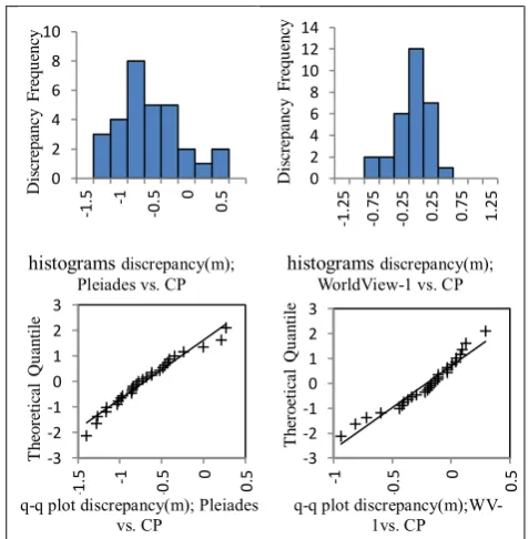
Regarding the errors, they are assumed to be random variables that are normally distributed. This assumption has been checked by testing the histogram normality using the q-q plot as shown in Figure 2.
histograms discrepancy(m);
Pleiades vs. CP histograms WorldView-1 vs. CPdiscrepancy(m);
q-q plot discrepancy(m); Pleiades
vs. CP q-q plot discrepancy(m);WV-1vs. CP
Figure 2. Original DSMs (Pleiades and WV-1) error distribution histograms and q-q plot against RTK check points.
5.2 Merging Using Maximum Likelihood Method
A Maximum Likelihood method is considered the traditional method for estimating the results using noisy input data, is also called the weighted average, and is based on the assumption that noise is normally distributed within the data. The Maximum Likelihood method is based on maximizing the probability associated with the estimated value of a pixel in the merged DSM; that is the error between the elevations in the input pixel (DSM̅̅̅̅̅̅ , ) and the corresponding estimated pixel (DSMk , ) is
required to be minimized.
|� =� √ � � −�� ;
|� =� √ � � −��
(4)
The estimated value of z is obtained by maximizing the likelihood function equation with respect to z (Mittelhammer, 2013), which leads to:
̅ �= argmax , |� =
� √ �
� −� � .
� √ �
� −�
� (5)
where: e is: is the exponential function
σ is: is the standard deviation which is representing the Digital Surface Model quality, and,
̅
�: is the value of the merged elevation usingMaximum Likelihood.
Equation 5 yields Equation 6, after it is simplified and maximized with respect to z, in order to get the Maximum Likelihood estimate for z. This method requires the variances to be known for each measurement, which in this case is represented by the square value of the quality (using RMSE in this situation) of each digital surface model. the detailed derivation of this equation is summarized in Sadeq, 2015.
̅ �= [� + �
� + �
] (6)
In other words, when the likelihood function and the observations z (i.e. z1, z2) are given, the estimated value is referred to as
̅
�. The model can be extended to cover more than two sensors, which is the case if there is more than one set of measurements:̅ �= [� + � + � + ⋯
� + � + � + ⋯
] (7)
5.3 Merging Using Bayesian Approach
The Maximum Likelihood approach can be considered to deal with each pixel individually and does not take into consideration
spatial correlation in the fused images’ pixels. For that reason the
DSM resulting from the fusion does not consider natural characteristics, such as smoothness, or other representations of the natural ground (Kotwal and Chaudhuri, 2013). So, in order to overcome the spatial correlation problem, it was necessary to introduce an a priori value which satisfactorily transformed the Maximum Likelihood value into a maximum a posteriori value, and transformed the problem from an ill-posed one into a well-posed one, by introducing an a priori value into the solution of
equation 2, which leads to the merged digital surface model (Beyerer et al., 2011).
In this section the Bayesian approach is used to invert the forward model equation 1; this model is used to express the digital surface model formation, blended with uncertainty, while incorporating a priori knowledge about the digital surface model (i.e. its morphological properties). The most important benefit in a Bayesian approach and which does not exist in the other methods, is that the effect of noise is reduced by using a suitable a priori value. As already mentioned, it is assumed the errors are random and they can be represented by a Gaussian distribution with mean equal to elevation of the used DSM and variance numerically linked to the uncertainty in the digital surface model, measured by evaluating the quality, using checkpoints, and then blunder is detected and eliminated.
According to the Bayesian equation, the merging is based on multiplying the likelihood by the a priori elevation; the likelihood is based on maximizing the probability. Recalling that the Bayesian rule, used to get the a posteriori probability, is represented by:
�| = |� � = � �ℎ × � � � � � (8)
then, recalling equation 2, and assuming that the sensor error is
normally distributed with mean z and variance σ2 , , σ (which represents the quality of the digital surface model) if there are two sensors:
= + � , � ~
, σ
(9)= + � , � ~
, σ
(10)The elevations predicted through maximizing entropy have associated probabilities. Suppose that the elevation error is normally distributed, that the mean error is equal to mean elevation, which is so in this case is , � , then the estimated a priori probability of the elevation, from (DSMk , , can be
based on a smoothed surface. This smoothing can be achieved by maximizing local entropy; three smoothed data sets are produced, based on a 3x3, a 5x5 and a 9x9 window respectively. For the two models being considered here, i.e. (DSMk x,y where k = 1 or k = 2. The Bayesian approach can be simplified to include only the likelihood and a priori data, and that , the normalization factor, can be eliminated since the situation is not dealing with finding the absolute value of the probability. Assuming there are only two sensors, this results in:
̂ ��= �� � | ,
= | , ~ − � −�� + � −�� + ���−� + ���−�
(11)
Simplifying the equation and minimizing the result by taking the log of equation 11, the result of the Maximum A Posteriori (probability) (or MAP) which represents the merged digital surface models can be obtained from the following expression:
̂
�� =[
� + � + � + �
� + � + � + �
]
(12)priori probability of the elevation, and then use the third data set (z3) in its original form, with the merged data set (ZMAP_old) in a weighted average operation, as shown in equation 13:
̂
��_ =[
� +� ��_��_
� + � ��_
]
(13)It is important to determine the quality of the a priori elevation, by using the below equation as shown by (Weng, 2002) :
� ��_ ��=� + �� � (14)
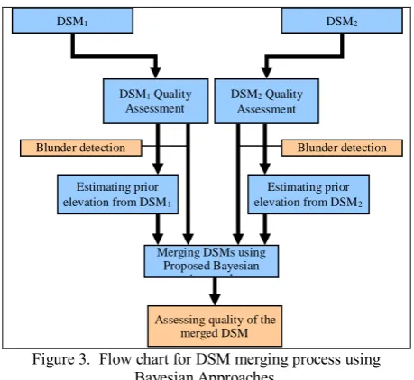
The above mentioned steps can be summarized through the flow chart blow that shows the steps of merging DSMs based on Bayesian approaches
Figure 3. Flow chart for DSM merging process using Bayesian Approaches.
5.4 Estimating the a priori using Maximum Entropy
The assumption that is made when constructing the a priori value is to build on the assumption that constructed building surfaces are smooth and have low roughness. This assumption can be quantified by using maximum entropy.
It is clear that entropy is representing the randomness in elevation variations which, consequently, can be employed to characterize the digital surface model. These characteristics can be used to manifest the representation of surface roughness, by assuming that the surface is smooth when the entropy is at the maximum and it is rough (or not smooth) when the entropy is lowest. Based on this assumption one can try to maximize the entropy by changing the value of the middle of the window.
Maximizing the entropy by assigning different values will give an elevation that can be considered as the value of the a priori elevation.
According to the earlier discussion about entropy and how entropy can be used to represent roughness, and as illustrated in Figure 5, maximum entropy is obtained when the probabilities are similar, and the uncertainty is high between the probabilities, i.e. the elevations are close to each other and the surface is smooth.
Figure 4. DSM shows different value of elevations used to represent the entropy (a) the entropy is low since the randomness in the elevations is high (b) the entropy is high
since the variance in the elevation is low.
The group of probabilities pij from p11 to pMN in a specific
window size MN, are represented by the value Hf. The equation 15 represents a one dimension signal, but it can be transformed to apply to a window:
��= ∑ ∑
= =
∗ (15)
where:
= , / ∑ ∑ ,
= =
(16)
The values of the heights have been transformed into probabilities within the specific window, MN. At each element of the window, the height probability has been evaluated by dividing each pixel value, f, by the total values of elevation within the specific window in order to find pij.
In order to determine the a priori elevation value, the window is generated each time the maximum entropy is determined for a specific elevation. The model that is used for determining the entropy is illustrated in Equation 17.
�̂ = �� max� ∏ � (17)
�
̂
in equation represents the maximum entropy.6. RESULTS, ANALYSES AND DISCUSSION
This section includes the evaluation of each created and merged DSM that has been generated from optical satellite imagery implementing the developed models. For evaluation purposes 31 check points have been used which were acquired by differential GNSS observations and are considered to be the ‘true’ ground elevations. Both quantitative and qualitative analyses have been used in this evaluation.
The merged DSMs can be classified into two types: Maximum Likelihood (i.e. weighted average) and Bayesian Merging.
Within Bayesian Merging there were three groups derived from the implemented window size used in estimating the a priori probability of elevation, based on maximising local entropy, namely 3x3, 5x5 and 7x7 windows. Each of them has been evaluated based on two different iteration loops in a ± 0.1m range and a± 0.25m range, using a 0.01m increment.
6.1 Statistical Assessment
The statistical tests that have been used in the merged DSM validation have been applied after eliminating blunders. Empirical equations, and statistical tests have been used in the quantitative evaluation , such as (RMSE) and ‘determination
coefficient’, r2 (Legates and McCabe, 1999).
DSM1 DSM2
DSM1 Quality Assessment
Blunder detection DSM2 Quality
Assessment
Blunder detection
Estimating prior elevation from DSM1
Estimating prior elevation from DSM2
Merging DSMs using Proposed Bayesian
Approach
It can be noticed that the errors (discrepancies), which are RMSE of the merged digital surface model with range ±0.1m is smaller than the RMSE of the merged digital surface model with the ±0.25m range for both the a priori probability of elevation obtained from the 3x3 and 5x5 windows, while the RMSE when the 7x7 window is used to obtain the a priori probability of elevation with the ±0.25m range was better than that achieved with ±0.1m range. The σ of error values were almost the same in all cases (i.e. all size windows and all increments for estimating a priori elevation).
The coefficient r2 has been used in order to test the correlation between the DSMs’ elevations and GCPs’ elevations. From the previous section it can be seen that the equation 12, represents the merged model using a Bayesian approach in the case when the measurements was limited to two digital surface models only.
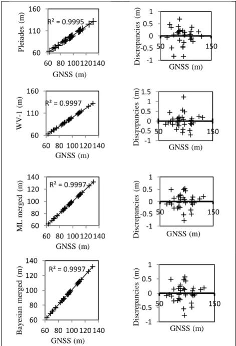
Figure 5. Comparison of the correlation and scatter plot for the
input data and merging results using Maximum Likelihood and Bayesian techniques against checkpoints (CPs). First row is for
Pleiades vs. Checkpoints, second row is for WV-1 vs. Checkpoints, third row is for Maximum Likelihood vs. Checkpoints, and fourth row is for Bayesian merging - range
±0.25m window 3x3 vs. Checkpoints.
It should be noted that the standard deviation of the error (or σ of
discrepancies), which can be considered to be an unbiased representation of error, has been reduced in all the merged DSMs
to be better than that for the original data. Initially it was 0.359m (Pleiades) and 0.320m (WorldView-1) and the merging has led it to be 0.306m in the worst case.
The error illustrated in Figure 5, shows the differences between the DSMs either from the original or a merged DSM and the
‘true’ values. This has been measured by taking the difference
from of the GCP elevations and the aforementioned DSMs at each checkpoint.
The Bayesian approach has considerable influence on imposing normality on the error distribution as can be seen from the plots of each type regardless of the window size and the iteration range used in looping for estimating the a priori probability of the elevation value. An analysis of the discrepancy scatter plots Figure 5, as recommended by Rusling and Kumosinski (1996) shows that all the values are randomly distributed which further validates the linear relationship between all sets of interpolated heights and their checkpoint values.
6.2 DSM Qualitative Assessment
In addition to the quantitative assessment, a qualitative assessment has been implemented. Different analyses were implemented, using visual inspection on generated profiles and slope maps from the DSMs.
6.2.1 Height comparison: Figure 6 shows the profiles that were produced at the merging stage, against the original profiles. The weighted average (Maximum Likelihood) approach enhances the DSM by removing irregularities in the underlying DSM and shows, graphically, that the WorldView-1 DSM has,
through the weighting process based on the DSM’s quality, more
influence on the underlying DSM than does Pleiades.
Figure 6. Profile for height assessment.
Due to variations in satellite geometry, it can be noticed from Figure 6 that there is a misregistration in the DSMs and consequently in the produced profile due to weak satellite geometry (Teo et al., 2010).
6.2.2 Slope Analysis: Further DSM assessment has been achieved by producing a slope map. In the analysis of the produced maps, Figure 7, it has been shown that the Bayesian approach has an active affect on smoothing the flat surfaces during the merging process. This can support the assumption that has been made during estimating the a priori probability of elevation used in the Bayesian approach.
(a) Pleiades DSM (b)Bayesian merged DSM Figure 7. 3D view showing the effect of merging over a flat
surfaced structure.
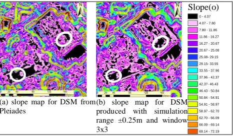
For further detailed qualitative validation, different slope maps have been produced either for the original DSMs or for the merged DSMs as shown in Figure 8, in order to find out the change in the surface slope between each stage.
(a) slope map for DSM from Pleiades
(b) slope map for DSM produced with simulation range ±0.25m and window 3x3
Slope(o)
Figure 8. Slope map analysis for merged DSMs, the white symbolization shows the effect of merging on removing the slope.
For further detailed analysis of the DSM’s slope map, Table 2 shows the statistics analysis for each slope map within the study area represented by the arithmetic mean and standard deviations of the slope values across the whole study.
Source of the DSM
WorldView-1 satellite imagery(A) 25.402 19.919
Pleiades satellite imagery(B) 27.740 21.199
Merging (A and B) with Maximum
Likelihood 25.292 19.495
Merging (A and B) with Bayesian range
±0.1m and 3x3window 25.279 19.628
Merging (A and B) with Bayesian
simulation range ±0.25m and 3x3window 25.220 19.515 Merging (A and B) with Bayesian
simulation range ±0.1m and 5x5window 25.196 19.725 Merging (A and B) with Bayesian
simulation range ±0.25m and 5x5window 25.037 19.617 Merging (A and B) with Bayesian
simulation range ±0.1m and 7x7window 25.135 19.778 Merging (A and B) with Bayesian
simulation range ±0.25m and 7x7window 25.892 19.705 Table 2. Merged and original slope map statistical analysis.
In the slope map analysis, the average slope of the merged DSMs using the Bayesian approaches (i.e. all used window sizes and variances) is less than that for the slopes of the merged DSM achieved using the Maximum Likelihood approach. Moreover, the arithmetic mean values decrease with increasing the window size or with increasing the range value, because with a higher increment value, the patch that is used to infer an a priori probability of elevation has become smoother. On the other hand, the standard deviations of slope across the whole study area for the merged DSMs are less than the original DSMs used in the merging. The standard deviation of the merged DSMs using the Maximum Likelihood method is less than the DSMs using Bayesian approaches. Moreover, the standard deviation of slope across the whole study area rose with increased window size, and for each window size the standard deviation is increased with increasing the range (e.g. with simulation range of ±0.25m rather than ±0.1m).
7. CONCLUSION
In this research a statistical approach, based on probabilistic methods, has been investigated for merging DSMs and enhancing building footprints. Due to increasing the sources for DSM construction, merging DSMs can reduce data redundancy while improving the quality of the data. The applied statistical tests have shown that merging using a Bayesian method can provide DSM results similar to those achieved using a Maximum Likelihood method for merging, and it can be used for its intended purpose. It was hoped to obtain a DSM that had better characteristics than the original. Noticeable improvements in accuracy cannot, theoretically, be achieved, and purely on the positional accuracy basis the unmerged WorldView-1 DSM offers the greatest accuracy, but a more complete model can be achieved, and an approach is offered which can be used to detect blunders in a contributing DSM. Also the Bayesian approach has helped to smooth the surface of the generated structures so it may represent the real surfaces found in urban areas better. It can be acknowledged that the effect of misregistration has not been
‘Bayesian methods for image fusion’, in Stathaki, T. (ed.) Image Fusion: Algorithms and Applications, Academic Press., pp. 157– 192.
Chen, C. and Yue, T. (2010) ‘A method of DEM construction and related error analysis’, Computers & Geosciences. Elsevier, 36(6), pp. 717–725.
Dowman, I. (2004) ‘Integration of LiDAR and IFSAR for mapping’, in International Archives of Photogrammetry and Remote Sensing. Istanbul, Turkey, pp. 90–100. Available at: http://eprints.ucl.ac.uk/11082/ (Accessed: 9 September 2014).
Feron, O. and Mohammad-Djafari, A. (2004) ‘A Hidden Markov
model for Bayesian data fusion of multivariate signals’, Journal of Electronic Imaging, 14(2), pp. 1–14. Available at: http://arxiv.org/abs/physics/0403149 (Accessed: 12 June 2014).
Ge, Z., Wang, B. and Zhang, L. (2007) ‘Remote sensing image
fusion based on Bayesian linear estimation’, Science in China Series F: Information Sciences, 50(2), pp. 227–240.
Gelman, A., Carlin, J., Stern, H. and Rubin, D. (2004) Bayesian data analysis. 2nd ed. Chapman & Hall/CRC.
Gheta, I., Heizmann, M. and Beyerer, J. (2008) ‘Bayesian Fusion
of Multivariate Image Series to Obtain Depth Information’, in
Proceedings of Fusion. Köln, pp. 1731–1737.
Hosford, S., Baghdadi, N., Bourgine, B., Daniels, P. and King,
C. (2003) ‘Fusion of airborne laser altimeter and RADARSAT
data for DEM generation’, in IGARSS 2003. 2003 IEEE International Geoscience and Remote Sensing Symposium. Proceedings (IEEE Cat. No.03CH37477). IEEE, pp. 806–808.
Kotwal, K. and Chaudhuri, S. (2013) ‘A Bayesian approach to
visualization-oriented hyperspectral image fusion’, Information Fusion. Elsevier B.V., 14(4), pp. 349–360.
Lee, S. H., Baek, S. and Shum, C. K. (2005) ‘Multi-temporal, multi-resolution data fusion for Antarctica DEM determination
using InSAR and altimetry’, in Geoscience and Remote Sensing
Symposium, 2005. IGARSS ’05. Proceedings. 2005 IEEE
International. IEEE, pp. 2827–2829.
Legates, D. R. and McCabe, G. J. (1999) ‘Evaluating the use of “goodness-of-fit” Measures in hydrologic and hydroclimatic
model validation’, Water Resources Research, 35(1), pp. 233– 241.
Li, Z. (1990) Sampling strategy and accuracy assessment for digital terrain modelling. (PhD Thesis),University of Glasgow.
Li, Z. (1992) ‘Variation of the accuracy of digital terrain models with sampling interval’, The Photogrammetric Record, 14(April), pp. 113–128.
Mascarenhas, N. D. A., Banon, G. J. F. and Candeias, A. L. B.
(1992) ‘Image Data Fusion under A Bayesian Approach’, in
[Proceedings] IGARSS ’92 International Geoscience and
Remote Sensing Symposium. IEEE, pp. 675–677.
Mittelhammer, R. C. (2013) Mathematical Statistics for Economics and Business. New York, NY: Springer New York.
Mohammad-Djafari, A. (2003) ‘A Bayesian Approach for Data
and Image Fusion’, in AIP Conference Proceedings. AIP, pp. 386–408.
Papasaika, H., Poli, D. and Baltsavias, E. (2009) ‘Fusion of
Digital Elevation Models from Various Data Sources’, in 2009 International Conference on Advanced Geographic Information Systems & Web Services. IEEE, pp. 117–122.
Papasaika-Hanusch, C. (2012) Fusion of Digital Elevation Models. PhD thesis, ETH Zurich.
Podobnikar, T. (2007) ‘DEM from various data sources and geomorphic details enhancement’, Proceedings of 5th Mountain Cartograpy Workshop, Bohinj, Slovenia. Zürich: International Cartographic Association, Commission on Mountain Cartography, pp. 189–199.
Punska, O. (1999) Bayesian Approaches to Multi-Sensor Data Fusion. (MSc Thesis) University of Cambridge.
Reuter, H., Strobl, P. and Mehl, W. (2011) ‘How to merge a DEM?’, Geomorphometry, pp. 87–90. Available at: http://www.geomorphometry.org/system/files/Reuter2011geom orphometry.pdf (Accessed: 17 June 2012).
Rusling, J. F. and Kumosinski, T. F. (1996) Nonlinear computer
modeling of chemical and biochemical data. Academic Press.
Saeedi, P. and Zwick, H. (2008) ‘Automatic building detection in
aerial and satellite images’, in IEEE10th International Conference on Control, Automation, Robotics and Vision, pp. 623–629.
Schultz, H., Riseman, E. M. and Stolle, F. R. (1999) ‘Error
detection and DEM fusion using self-consistency’, in Proceedings of the Seventh IEEE International Conference on Computer Vision. IEEE, pp. 1174–1181 vol.2.
Shi, X. and Manduchi, R. (2003) ‘A Study on Bayes Feature Fusion for Image Classification’, in 2003 Conference on Computer Vision and Pattern Recognition Workshop. IEEE, pp. 95–95.
Teo, T. A., Chen, L. C., Liu, C. L., Tung, Y. C. and Wu, W. Y.
(2010) ‘DEM-aided block adjustment for satellite images with
weak convergence geometry’, IEEE Transactions on Geoscience and Remote Sensing, 48(4 PART 2), pp. 1907–1918.
Wegmüller, U., Wiesmann, A. and Santoro, M. (2010) ‘Merging of an EET CInSAR DEM with the SRTM DEM’, Gamma Remote, Sensing Ag.
Weng, Q. (2002) ‘Quantifying uncertainty of digital elevation models derived from topographic maps’, Richardson, D.E. and van Oosterom, O., editors, Advances in spatial data handling: 10th International Symposium on Spatial Data Handling, Berlin: Springer, pp. 403–408. Available at: http://link.springer.com/chapter/10.1007/978-3-642-56094-1_30 (Accessed: 13 November 2014).
Zaniboni, G. and Mascarenhas, N. (1998) ‘Fusão bayesiana de
imagens utilizando coeficientes de correlação localmente
adaptáveis’, Simpósio Brasileiro de Sensoriamento Remoto, 9. (SBSR), pp. 1003–1014.
Zhang, B. and Smith, W. (2010) ‘From Where to What: Image Understanding Through 3-D Geometric Shapes’, in ASPRS 2010 Annual Conference.
Zhang, J. (2010) ‘Multi-source remote sensing data fusion: status