Birth Order, Educational Attainment,
and Earnings
An Investigation Using the PSID
Jasmin Kantarevic
Stéphane Mechoulan
a b s t r a c t
We examine the implications of being early in the birth order, and whether a pattern exists within large families of falling then rising attainment with respect to birth order. Unlike other studies using U.S. data, we go beyond grade for age and look at racial differences. Drawing from OLS and fixed effects estimations, we find that being first-born confers a significant educa-tional advantage that persists when considering earnings; being last-born confers none. These effects are significant for large Black families at the high school level, and for White families of any size at both high school and college levels.
I. Introduction
Whether birth order affects performance has been an open empirical question for decades. In this study, we examine whether being early in the birth order implies a distinct educational and professional advantage, and whether within large families a pattern exists of falling then rising attainment with respect to birth order.
The empirical results presented here, drawn from the Panel Study of Income Dynamics (PSID), show that being first-born does confer an advantage, while being last-born confers none. In particular, we stress the importance of controlling for the age of the mother at childbirth. The age of the mother at childbirth is positively cor-related with a child’s education. At the same time, it is mechanically, positively
Jasmin Kantarevic is a senior economist at the Ontario Medical Association and a research affilate at the Institute for Labor Studies (IZA). Stéphane Mechoulan is an assistant professor of economics at the University of Toronto. The authors thank Gadi Barlevy, Chris Jepsen, Nancy Qian, Imran Rasul, seminar participants at the University of Toronto and UQAM, and two anonymous referees for valuable comments and suggestions. The data used in this article can be obtained beginning March 2007 through February 2010 from Jasmin Kantarevic, Ontario Medical Association, 525 University Ave, Suite 300, Toronto, Ontario, M5G 2K7 Canada, Jasmin_Kantarevic@OMA.ORG.
[Submitted February 2005; accepted December 2005]
ISSN 022-166X E-ISSN 1548-8004 © 2006 by the Board of Regents of the University of Wisconsin System
correlated with a child’s birth order. The omitted variable bias results in a clear offset of the birth-order effect and represents a simple yet unrecognized source of model misspecification.
A causal interpretation of the previous analysis would be premature. Total number of siblings, the age of the mother at childbirth, and other covariates such as parental education are likely correlated with unobservable socioeconomic characteristics. In particular, the precise causal determination of early motherhood on children’s aca-demic outcomes has received considerable attention (for example, Geronimus, Korenman, and Hillemeier 1994; Hofferth and Reid 2002; Lopez-Turley 2003), fol-lowing an even larger debate on the consequences of early pregnancy on mothers them-selves.1Yet, even if early motherhood does not causelower educational attainment for a child, it is still possible that first-borns perform relatively better, conditional on early motherhood.
It would be very difficult to find compelling instrumental variables for all our potentially endogenous regressors. Therefore, to provide additional credibility to our results, we use a fixed effects (FE) model, which by construction removes variables that are constant withina family. As such, we take care of unobserved family-level heterogeneity. The results on birth order are broadly consistent with our initial ones.
The PSID enables us to check whether those patterns vary by ethnicity and whether the effect we find is in the higher educational realm, where financing matters. In partic-ular, we investigate whether birth order influences secondary or postsecondary education. We find that birth-order effects are relatively stronger for White families. Furthermore, both ordinary least squares (OLS) and FE estimations show that the first-born lead is already revealed at the high school stage.2Yet, the exact mechanism through which first-borns appear to be advantaged is not fully identifiable from our data.
Lastly, the PSID gives us an opportunity to track outcomes over a longer period than just school years. Therefore, as a final check of the robustness of the results, we estimate the impact of birth order on hourly earnings. The same patterns emerge, so that when we omit the age of the mother at birth, we find no effect, whereas when we include it, we find a strong positive influence of birth order on hourly earnings. We do not find compelling evidence of differential birth-order effects on earnings between White and Black families.
Our work relates to an active literature in the economics of the family that is fun-damental to our understanding of the intra-household allocation of resources.3Our results are consistent with those found by Black, Devereux, and Salvanes (2005) in Norway, Booth and Kee (2005) in the United Kingdom, and Conley and Glauber (2004) in the United States. Yet unlike Conley and Glauber (2004), we are able to go beyond grade for age.
The Journal of Human Resources
756
1. Obviously, the age of the mother at childbirth is linked to a number of variables that should affect a child’s educational attainment. Younger mothers are more likely to be single, have less human capital, etc. Also, adverse effects of unplanned motherhood may dissipate over time (Bronars and Grogger 1993).
2. Specifically, birth-order effects are significant for large Black families at the high school level only, and for White families of any size these effects are significant at both the high school and college level. We also look at the probability of repeating a grade conditional on high school completion, which does not seem sig-nificantly influenced by birth order.
Our contribution is perhaps most closely related to the work of Hanushek (1992), who used a sample of school children from low-income Black families in early 1970s Indiana. Hanushek’s paper advances that while being early in the birth order implies a distinct advantage, it is entirely due to the higher probability of coming from a small family. Following Lindert (1977), the paper also highlights, within large families, a distinct and sizeable pattern of falling and then rising attainment with respect to birth order, to the point that it becomes best to be last-born. In contrast to Hanushek, our sample is more representative: We are thus able to examine longer-run outcomes and we also look at racial differences. Our empirical results first present a close version of Hanushek’s findings before challenging their robustness, by introducing age of mother at birth in the model, and running fixed effects estimations.
The rest of the paper is organized as follows. Section II presents our data. Section III shows how birth order affects various educational outcomes through different esti-mation strategies. Section IV then extends the analysis to earnings. Finally, Section V concludes.
II. Description of the Data
Our data come from the Childbirth and Adoption History File (CAHF), a special supplemental file of the PSID. The CAHF covers eligible people4 living in a PSID family at the time of the interview in any wave from 1985 through 2001.
The population examined here (henceforth the “index persons”) consists of all those for whom the CAHF sample contains records of the childbirth histories of at least one of their parents. The CAHF allows us to compile information on their birth order and the total number of children that their parent(s) report(s).
The index persons with missing information on their birth order or for whom the number of siblings is not ascertained are necessarily excluded from the sample. To ensure that all mothers have completed their fertility so that we correctly identify the total number of siblings, we further limit the sample to those index persons whose mother was older than 44 in the last year she reported.
Siblings are defined based on the childbirth histories of mothers.5In addition to the birth order and the number of siblings of the index persons, we have obtained additional demographic information on them and their parents from other PSID files using the unique individual identifiers that are present in the PSID main and supple-mental files.
Notably, the PSID suffers from an important attrition bias. More educated people tend to stick with the questionnaire over longer periods of time; thus, it appearsthat
4. Eligible persons are defined as heads or wives of any age and other members of the family unit aged 12–44 at the time of the interview. These individuals are asked retrospective questions about their birth and adoption histories at the time of their first interview. In each succeeding wave these histories are updated. 5. The sample shrinks by 30 percent if siblings are defined based on the childbirth histories of fathers. In case both parents report, we were able to identify between siblings and half siblings; however, this distinc-tion did not change any of our results. We include a variable expressing whether both parents report in our regressions.
Table 1
Descriptive Statistics
Variable Standard
Index individual Observations Mean Deviation Minimum Maximum
Years of completed education 8,147 12.62 2.13 1 17
Percent completed high school 8,147 0.82 — 0 1
Log hourly earnings in 2001 3,028 2.67 0.71 −1.2 5.99
Age (in 2001) 8,318 38.57 8.76 25 89
Percent male 8,318 0.5 — 0 1
Percent White 8,318 0.47 — 0 1
Number of siblings 8,318 4.86 2.72 2 16
Percent first-born 8,318 0.27 — 0 1
Percent second-born 8,318 0.27 — 0 1
Percent third-born 8,318 0.17 — 0 1
Percent fourth-born 8,318 0.11 — 0 1
Percent fifth-born 8,318 0.07 — 0 1
Information on all siblings 8,318 0.56 — 0 1
Both parents report the childbirth 8,318 0.60 — 0 1
Family income
Age 1–6 2,695 13,639 9,283 508 97,660
Age 7–14 4,576 19,993 17,360 1,173 255,393
Age 1–14 3,474 18,850 14,026 1,092 178,480
Mother continuously married
Age 1–6 8,318 0.25 — 0 1
Age 7–14 8,318 0.36 — 0 1
Age 1–14 8,318 0.21 — 0 1
Mother
Age at birth 8,292 26.18 5.88 15 48
Years of completed education 8,102 11.03 3.02 1 20
Father
Age at birth 5,000 29.32 6.54 17 60
Years of completed education 4,892 11.13 3.67 1 17
Includes index persons who have at least one sibling, who are 25 years or older in 2001, and whose mother is at least 44 years old in the last year she reported. The number of distinct families is 3,112.
The Journal of Human Resources
Kantarevic and Mechoulan 759
education is decreasing over cohorts, which is of course untrue according to the U.S. Census. Because a first-born is older than other siblings by definition, this alone could, in theory, produce a spurious positive impact of being first-born on education. We have checked that this problem is of no consequence for our results.6
The summary statistics of our sample are presented in Table 1. The detailed description of variables is relegated to Appendix 1. We found more than 8,000 index persons (from more than 3,100 distinct families) older than 24 in 2001, with at least one other sibling, and whose mother has completed her fertility. This is to be con-trasted with Conley and Glauber (2004) who use larger sample from the U.S. Census, but focus only on children under the age of 20 living at home.
The main dependent variable—years of completed education—has an average of 12.62 years.7About 82 percent of those selected index persons have at least 12 years of
education, that is to say, have completed high school.8Our measure of earnings—log
hourly wage in 2001—shows an average corresponding to $14.5/hour. However, the information on hourly wages or salary income is not available for most index persons.
The average age in our sample is 39. About half of respondents are male and 47 percent are White. The average number of siblings is 4.86. This high number is con-sistent with the PSID oversampling minorities and low-income populations. Fifty-six percent of the index persons have all their siblings reporting, and 60 percent have both their parents reporting their childbirth history.
We improved our analysis by including important observed family level-effects that vary across parity: family income, and whether the mother is married. Whenever available, we constructed the corresponding information for each of the first 14 years
of life of each index person.9 The main limitation is that information on family
income cannot be recovered for many index individuals.
Lastly, we include two variables describing characteristics of index individuals’ par-ents, namely education (11 years for both mother and father on average) and the age of the parents at birth of index persons (26 for mothers and 29 for fathers on average).
III. Methods and Results
A. The First-Born Effect
We first use an OLS estimation with robust standard errors clustered by family unit (identified by the mother), which relaxes the independence assumption between the
6. The regressions presented in this article contain age controls that separate cohort from birth order effects. 7. A more appropriate variable would be education at age 25. However, the number of observations avail-able would drop considerably and we would not be avail-able to run estimations bysibling size. All of our other results when running estimations that control forsiblings size hold when replacing education with education at age 25 for those where such information can be traced.
8. A negligible fraction of those who declare a certain education level at some point in their life declare less education later. Removing such observations did not alter our results. We therefore choose the latest educa-tion level reported as our variable of interest.
The Journal of Human Resources
760
error terms and requires only that the observations be independent across clusters.10
In Table 2, we first test the hypothesis that being early in the birth order implies a dis-tinct advantage that is entirely due to the higher probability of coming from a small family.
Columns 1 and 2 of Table 2 reject that claim but help us understand why it may have been made. In Column 1, we omit the number of siblings; therefore, the signif-icant coefficient on first-born reflects not only the birth order effect but also the prob-ability of coming from a small family. In Column 2, the inclusion of the number of siblings leaves the coefficient on first-born insignificant.
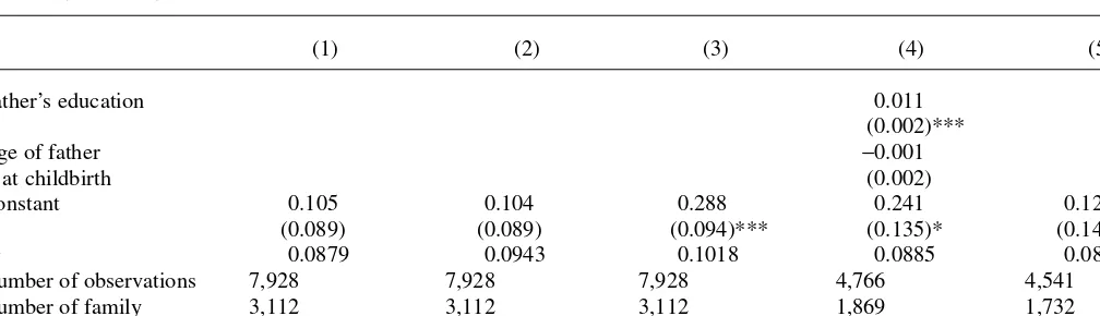
In Column 3, we include age of the mother at childbirth and find a positive and highly significant effect of being first-born on years of education. This effect is con-firmed when including the father’s characteristics in Column 4, where both a father and a mother report. Often, not all siblings report; this is especially the case for large fam-ilies. To check if we are biasing our results by including such families, in Column 5 we restrict our attention to families with complete information on all siblings. The findings are similar there too, further showing that they could not be driven by selective attri-tion within families by birth order. In all specificaattri-tions, we find a stronger effect among White families.
The results presented here are for the impact of being first-born in families of more than one child. This particular procedure takes advantage of the full size of our sam-ple and can be useful when there are not enough observations to run separate estima-tions for different siblings’ sizes.11We see that it allows us to reveal a significant and
robust birth order effect.
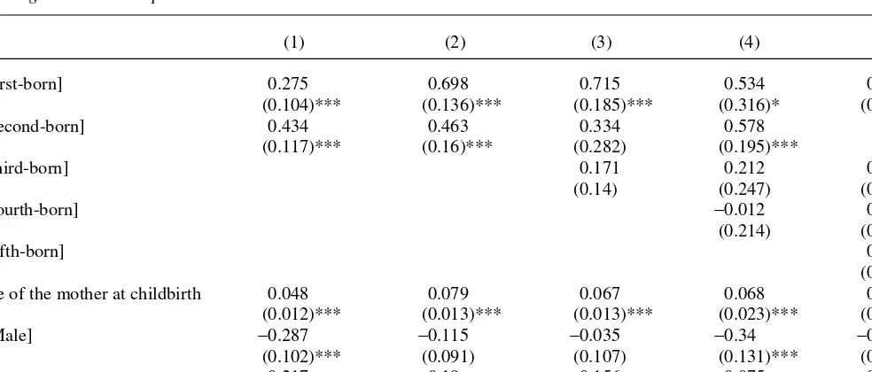
However, we still obtain similar results when looking at individual birth order effects by siblings’ size in Table 3, where all specifications include age of the mother at childbirth. Although large families show higher birth order point estimates, the effect is present in two-sibling families as well. Note that the coefficient on first-born is only weakly significant in Column 4—families of five siblings—likely because of the small sample size.
The reason why the inclusion of the age of the mother at childbirth makes the coef-ficient on first-born larger in magnitude and more significant is clear: The age of the mother at childbirth is mechanically, positively correlated with birth order, and even more strongly across large families. Conversely, we see that it is positively correlated with a child’s education. Then, if having a high birth order carries a negative impact on education, the two effects of birth order and age of the mother at childbirth com-pete against one another. Therefore the coefficient on first-born in Table 2, Column 2 reflects an omitted variable bias. The results hold for both males and females, for mothers with or without more than a high school education. We also found that spac-ing between births, be it that of the first-born child with respect to the second-born or to the last-born child, does not alter the conclusions either. Additional OLS regres-sions confirmed that the effect is significantly present among White families of any
10. We also used random effects procedures, but because they yield almost identical results as those with the family clustered standard errors, those are not reported.
Kantare
vic and Mechoulan
761
Table 2
OLS Regression with Dependent Variable: Education
(1) (2) (3) (4) (5)
d[first-born] 0.162 0.012 0.288 0.239 0.268
(0.068)** (0.069) (0.072)*** (0.098)** (0.084)***
Total number of siblings −0.104 −0.121 −0.108 −0.125
(0.015)*** (0.015)*** (0.019)*** (0.029)***
Age of mother at childbirth 0.058 0.061 0.065
(0.005)*** (0.011)*** (0.008)***
d[Male] −0.205 −0.21 −0.226 −0.186 −0.159
(0.047)*** (0.046)*** (0.046)*** (0.058)*** (0.057)***
Age 0.121 0.159 0.162 0.143 0.087
(0.027)*** (0.027)*** (0.027)*** (0.039)*** (0.040)***
Age2 −0.001 −0.001 −0.001 −0.001 −0.003
(0.0003)*** (0.0003)*** (0.0003)*** (0.001)** (0.0001)
d[White] 0.119 −0.003 −0.099 −0.295 −0.107
(0.072)* (0.073) (0.071) (0.087)*** (0.098)
d[first-born] ×d[White] 0.126 0.193 0.184 0.286 0.172
(0.092) (0.092)** (0.092)** (0.115)** (0.104)*
Mother’s education 0.213 0.198 0.199 0.114 0.236
(0.012)*** (0.012)*** (0.012)*** (0.017)*** (0.018)***
d[all siblings report] 0.261 0.096 0.181 0.144
(0.068)*** (0.069) (0.069)*** (0.089)
d[both parents report] 0.523 0.553 0.520 0.533
(0.063)*** (0.062)*** (0.061)*** (0.081)***
Father’s education 0.125
(0.012)***
Age of father at childbirth 0.006
(0.009)
Constant 6.713 6.717 5.073 5.162 5.848
(0.528) (0.531)*** (0.541)*** (0.775)*** (0.776)***
R2 0.1578 0.1691 0.1889 0.2009 0.1982
Number of observations 7,928 7,928 7,928 7,766 4,541
Number of family clusters 3,112 3,112 3,112 1,869 1,732
(1)–(5): all mothers have completed their fertility (age > 44), all respondents assumed to have completed their education (age > 24) and have at least one other sibling. (4): d[both parents report] = 1 and (5): d[complete info on all siblings] = 1
The Journal of Human Resources
762
Table 3
OLS Regression with Dependent Variable: Education
(1) (2) (3) (4) (5)
d[first-born] 0.275 0.698 0.715 0.534 0.915
(0.104)*** (0.136)*** (0.185)*** (0.316)* (0.236)***
d[second-born] 0.434 0.463 0.334 0.578
(0.117)*** (0.16)*** (0.282) (0.195)***
d[third-born] 0.171 0.212 0.368
(0.14) (0.247) (0.175)**
d[fourth-born] −0.012 0.466
(0.214) (0.152)***
d[fifth-born] 0.221
(0.133)*
Age of the mother at childbirth 0.048 0.079 0.067 0.068 0.07
(0.012)*** (0.013)*** (0.013)*** (0.023)*** (0.013)***
d[Male] −0.287 −0.115 −0.035 −0.34 −0.033
(0.102)*** (0.091) (0.107) (0.131)*** (0.087)***
Age 0.217 0.19 0.156 0.075 0.167
Kantare
vic and Mechoulan
763
Age2 0.002 0.002 0.002 3
×10−4 0.002
(7×10⁻⁴)*** (7
×10−4)** (6
×10−4)** (5
×10−4) (8
×10−4)**
d[White] 0.119 −0.124 4×10⁻⁵
−0.03 −0.114
(0.12) (0.13) (0.13) (0.181) (0.137)
Mother’s education 0.257 0.25 0.179 0.124 0.182
(0.025)*** (0.026)*** (0.023)*** (0.035)*** (0.022)***
d[all siblings report] 0.147 0.212 −0.066 0.351 0.21
(0.154) (0.136) (0.128) (0.178)** (0.149)
d[both parents report] 0.241 0.612 0.755 0.542 0.371
(0.118)** (0.118)** (0.126)*** (0.189)*** (0.127)***
Constant 3.339 2.694 4.258 6.607 4.12
(1.148)*** (1.184)** (1.011)*** (1.293)*** (1.415)***
R2 0.185 0.21 0.19 0.114 0.127
Number of observations 1,398 1,705 1,444 959 2,422
Number of family clusters 913 811 542 308 538
(1)–(5): all mothers have completed their fertility (age > 44), all respondents assumed to have completed their education (age > 24). (1)–(5): Families of 2, 3, 4, 5, and 6 and above siblings respectively.
The Journal of Human Resources
764
size greater than one, whereas it is only present within large families among Blacks. Therefore, the ethnic differential disappears when considering large families only.
As noted earlier, a causal interpretation of the age of the mother at childbirth would hinge on the assumption of its exogeneity. Without instrumental variables or a treat-ment versuscontrol quasi experiment, it is difficult to draw conclusions.12The age of
the mother at childbirth, itself positively correlated with birth order, could easily proxy for other unobserved variables such as level of human capital and parental resources.13
To address this problem, our fixed-effect estimation (Table 4a and b) removes fam-ily characteristics and unobserved famfam-ily-level heterogeneity.14Family fixed effects
address family unobservables to the extent that they are constant over time. While we try to incorporate observables that vary across birth order to affirm the robustness of our results, we are constrained by the availability of such variables in the data set.
Unfortunately, the coefficients on age or on age of the mother at childbirth are unin-formative in those fixed effects regressions. Deviations from family means for age convey the same information as deviations from family means for age of mother at childbirth. We thus do not provide separate estimations with age and age of mother at childbirth. The age of the mother at first childbirth is certainly relevant, but here, it is differenced out. Still, to assess this issue better, we ran separate regressions, split-ting the sample by maternal age.15To summarize, the following results are robust to
excluding mothers who first gave birth as teens, but we do not have enough observa-tions to meaningfully run the fixed effects regressions by sibling size on that latter group.
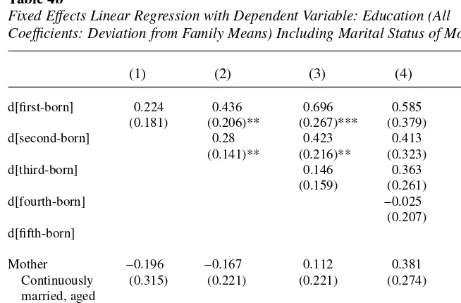
In Tables 4a and 4b, the fixed effects estimations that only control for age and gen-der confirm the previous results for the most part.16We also provide estimations
includ-ing the marital status of the mother17during the child’s first 14 years:18The results do
not change by much.19Clearly, the suggestion that first-borns are most likely to live
12. Also, while it is possible in the context of larger samples to instrument for siblings size—using twin births (Black, Devereux, and Salvanes 2005) or using the fact that parents of two same sex children are more likely to have a third child (Conley and Glauber 2004)—one cannot instrument for birth order per se. 13. This is further evidenced by the fact that including a dummy variable indicating whether the mother was married at the time of childbirth instead of (and, obviously, also along with) age of mother at childbirth also results in highly significant birth order coefficients. Results are available upon request.
14. However, it is worth noting that those fixed effects do not solve all endogeneity issues. For example, it may be the case that first-born “quality” is affecting subsequent fertility. We thank an anonymous referee for pointing out this caveat.
15. We thank an anonymous referee for this suggestion.
16. In Column 1—families of two siblings—the coefficient on first-born becomes significant at the 10 per-cent level when including index persons of 23 and 24 years of age, suggesting the nonsignificance when restricting at age 25 stems from a small sample size. Separate FE regressions for White and Black families confirmed the ethnic differentials found earlier.
17. We tried two definitions: number of years married/number of years considered in the age group, and = 1 if continuously married over the years considered in the age group, 0 otherwise. Since the results on birth order do not change qualitatively with either of those, we only report the results with the latter definition. 18. We also ran similar estimations with different age ranges and obtained similar results.
Kantarevic and Mechoulan 765
Table 4a
Fixed Effects Linear Regression with Dependent Variable: Education (All
Coefficients: Deviation from Family Means) Not Including Marital Status of Mother
(1) (2) (3) (4) (5)
d[first-born] 0.216 0.437 0.683 0.594 0.477
(0.181) (0.206)** (0.265)*** (0.379) (0.224)**
d[second- 0.282 0.412 0.421 0.199
born] (0.141)** (0.214)* (0.323) (0.195)
d[third- 0.138 0.361 0.055
born] (0.159) (0.261) (0.172)
d[fourth- −0.031 0.181
born] (0.207) (0.149)
d[fifth- −0.012
born] (0.125)
Observations 1,422 1,743 1,477 922 2,487
groups 934 835 562 388 573
Table 4b
Fixed Effects Linear Regression with Dependent Variable: Education (All Coefficients: Deviation from Family Means) Including Marital Status of Mother
(1) (2) (3) (4) (5)
d[first-born] 0.224 0.436 0.696 0.585 0.492
(0.181) (0.206)** (0.267)*** (0.379) (0.226)**
d[second-born] 0.28 0.423 0.413 0.212
(0.141)** (0.216)** (0.323) (0.197)
d[third-born] 0.146 0.363 0.063
(0.159) (0.261) (0.173)
d[fourth-born] −0.025 0.188
(0.207) (0.149)
d[fifth-born] −0.016
(0.125)
Mother −0.196 −0.167 0.112 0.381 −0.105
Continuously (0.315) (0.221) (0.221) (0.274) (0.178)
married, aged 1–14
Number of 1,422 1,743 1,477 999 2,487
observations
Number of 934 835 562 328 573
groups
The Journal of Human Resources
766
their critical development years in a stable household, as opposed to later-borns who may experience the divorce of their parents, cannot entirely explain the first-born advantage. At the same time, the persistence of birth-order effects naturally poses the problem of their origin.
The literature is not able to distinguish between different theories on the topic of birth order. For example, schooling circumstances play a large role in educational out-comes and may be related to birth order.20Our analysis is limited in the sense that it
cannot discriminate between many competing hypotheses on why birth order appears to be important.21
Nevertheless, we checked whether what appears as a first-born advantage predom-inantly comes from financial constraints, for example, parents sending their first-born to college and running out of money for the following siblings. Conley offers the fol-lowing argument: “[I]n terms of parental investment, the cup starts to run dry as we go down the line. . . . Parental resources, it appears, are allotted on a first come, first-served basis.”22Yet, if it turns out that first-borns perform better beforehand, then a
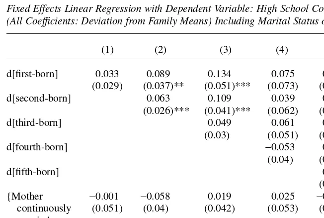
theory based on budget constraints cannot fully account for our results. In Tables 5–7, we estimate the probability of completing high school, following the same methodol-ogy as in Tables 2–4. We find that first-borns have a higher probability of completing high school than later born siblings.
Specifically, Table 5 shows again that the first-born effect is not an artifact of fam-ily size; that it increases in magnitude and significance when including age of mother at birth; that it is robust to including characteristics of father and to restricting the sample to families in which all siblings report. Table 6 shows that these results also hold when regressions are estimated separately by family size (except for families of five, presumably because of the small sample size). Tables 7a and 7b are the counter-parts of Tables 4a and 4b. Fixed effects regressions controlling for age and gender support the results found in Tables 5 and 6.23
Also, we estimated education at age 18 conditional on high school completion (at 18 or older) to see if later-borns are more likely to repeat grades, which would sup-port a theory of birth-order effects based on cognitive development differences. We did not find any evidence for this. However, the small sample size resulting from selecting index persons with available information at age 18 warrants some caution.
Finally, we found evidence, among White families only, that conditional on com-pleting high school, first-borns are more likely to receive postsecondary education. Yet for all races, conditional on postsecondary education, we found no clear advan-tage to being first-born.24In summary, financial constraints do seem to play a role, but
some factors early in life contribute to the first-born premium puzzle.
20. We thank an anonymous referee for this point.
21. We refer the reader to the survey of those theories presented in Black, Devereux, and Salvanes (2005). 22. Conley (2004), p. 69.
Kantare
vic and Mechoulan
767
Table 5
OLS Regression with Dependent Variable: High School Completion
(1) (2) (3) (4) (5)
d[first-born] 0.044 0.024 0.055 0.039 0.044
(0.014)*** (0.014)* (0.014)*** (0.018)** (0.017)***
Total number of 0.014 0.016 0.011 0.012
siblings (0.003)*** (0.003)*** (0.004)*** (0.005)***
Age of the mother 0.006 0.007 0.005
at childbirth (0.0001)*** (0.002)*** (0.001)***
d[Male] 0.047 0.048 0.049 0.047 0.037
(0.009)*** (0.009)*** (0.009)*** (0.009)*** (0.010)***
Age 0.024 0.029 0.029 0.032 0.023
(0.004)*** (0.004)*** (0.004)*** (0.007)*** (0.007)***
Age2 0.0002 0.0003 0.0002 0.0003 0.0002
(5×10⁻⁵)*** (5
×10−5)*** (5
×10−5)*** (8
×10−5)*** (8
×10−5)***
d[White] 0.005 0.012 0.023 0.042 0.019
(0.014) (0.014) (0.014)* (0.017)** (0.019)
d[first-born] ×d 0.015 −0.005 −0.006 0.011 0.006
[White] (0.0175) (0.017) (0.017) (0.021) (0.021)
Mother’s education 0.027 0.026 0.026 0.015 0.026
(0.002)*** (0.002)*** (0.002)*** (0.003)*** (0.003)***
d[complete info 0.035 0.094 0.022 0.029
on all siblings] (0.013)*** (0.012)*** (0.013) (0.015)*
d[both parents report] 0.09 0.094 0.090 0.097
The Journal of Human Resources
768
Table 5 (continued)
(1) (2) (3) (4) (5)
Father’s education 0.011
(0.002)***
Age of father −0.001
at childbirth (0.002)
Constant 0.105 0.104 0.288 0.241 0.129
(0.089) (0.089) (0.094)*** (0.135)* (0.141)
R2 0.0879 0.0943 0.1018 0.0885 0.0855
Number of observations 7,928 7,928 7,928 4,766 4,541
Number of family 3,112 3,112 3,112 1,869 1,732
clusters
(1)–(5): all mothers have completed their fertility (age > 44), all respondents assumed to have completed their education (age > 24) and have at least one other sibling. (4): d[both parents report] = 1 and (5): d[complete info on all siblings] = 1
Kantare
vic and Mechoulan
769
Table 6
OLS Regression with Dependent Variable: High School Completion
(1) (2) (3) (4) (5)
d[first-born] 0.038 0.084 0.09 0.031 0.122
(0.018)** (0.025)*** (0.036)** (0.053) (0.049)**
d[second-born] 0.071 0.08 2×10⁻⁴ 0.022
(0.022)*** (0.031)*** (0.051) (0.044)
d[third-born] 0.031 0.012 0.035
(0.028) (0.041) (0.037)
d[fourth-born] 0.061 0.041
(0.037) (0.033)
d[fifth-born] 0.007
(0.028)
Age of the mother at childbirth 0.003 0.004 0.009 0.008 0.011
(0.002)* (0.002)* (0.003)*** (0.004)** (0.003)***
d[Male] −0.03 −0.041 0.007 −0.094 −0.082
(0.016)* (0.016)** (0.02) (0.026)*** (0.018)***
Age 0.028 0.028 0.051 0.012 0.037
(0.007)*** (0.009)*** (0.01)*** (0.008) (0.011)***
Age2 3
×10−4 3
×10−4 5
×10−4 8
×10−5 4
×10−4
(9×10⁻⁵)*** (10−5)*** (10−5)*** (9
×10−5) (10−4)***
d[White] 0.012 0.124 0.049 0.033 0.022
(0.021) (0.023) (0.026)* (0.034) (0.028)
Mother’s education 0.024 0.025 0.027 0.018 0.027
The Journal of Human Resources
770
Table 6 (continued)
(1) (2) (3) (4) (5)
d[all siblings report] −0.011 0.03 −0.034 0.059 0.037
(0.025) (0.024) (0.024) (0.034)* (0.03)
d[both parents report] 0.045 0.076 0.125 0.088 0.098
(0.019)** (0.022)*** (0.027)*** (0.036)** (0.026)***
Constant 0.115 0.254 0.927 0.026 0.644
(0.16) (0.2) (0.2)*** (0.234) (0.261)**
R2 0.076 0.084 0.138 0.078 0.088
Number of observations 1,398 1,705 1,444 959 2,422
Number of family clusters 913 811 542 308 538
(1)–(5): all mothers have completed their fertility (age > 44), all respondents assumed to have completed their education (age > 24). (1)–(5): Families of 2, 3, 4, 5, and 6 and above siblings respectively.
Table 7a
Fixed Effects Linear Regression with Dependent Variable: High School Completion (All Coefficients: Deviation from Family Means) Not Including Marital Status of Mother
(1) (2) (3) (4) (5)
d[first-born] 0.033 0.089 0.132 0.076 0.124
(0.029) (0.037)** (0.051)*** (0.073)
(0.051)**
d[second-born] 0.064 0.107 0.039 0.029
(0.026)*** (0.041)*** (0.062) (0.045)
d[third-born] 0.048 0.061 0.047
(0.03) (0.05) (0.039)
d[fourth-born] −0.054 0.049
(0.04) (0.034)
d[fifth-born] 0.004
(0.029)
Observations 1,422 1,743 1,477 999 2,487
groups 934 835 562 328 573
Table 7b
Fixed Effects Linear Regression with Dependent Variable: High School Completion (All Coefficients: Deviation from Family Means) Including Marital Status of Mother
(1) (2) (3) (4) (5)
d[first-born] 0.033 0.089 0.134 0.075 0.129
(0.029) (0.037)** (0.051)*** (0.073) (0.052)***
d[second-born] 0.063 0.109 0.039 0.033
(0.026)*** (0.041)*** (0.062) (0.045)
d[third-born] 0.049 0.061 0.049
(0.03) (0.051) (0.039)
d[fourth-born] −0.053 0.051
(0.04) (0.034)
d[fifth-born] 0.004
(0.028)
{Mother −0.001 −0.058 0.019 0.025 −0.035
continuously (0.051) (0.04) (0.042) (0.053) (0.041)
married, age 1–14}
Observations 1,422 1,743 1,477 999 2,487
Groups 934 835 562 328 573
The Journal of Human Resources
772
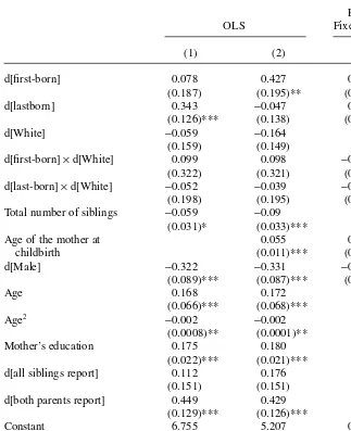
B. The “Last-Born Effect” in Large Families
We now test the hypothesis that within large (more than five siblings) families, the last-borns do better than the middle-last-borns, who in turn do worst. There is some support in the literature for a so-called “crunch in the middle” effect:25This nonlinear pattern was also
advanced by Hanushek (1992) and in the context of time allocation, by Lindert (1977). There are many ways to replicate these findings. Short of enough observations for each family size when family size is very large, the variables of interest chosen in Table 8 are dummies indicating whether a child is first-born and whether a child is last-born.
When omitting the age of mother at childbirth in Column 1, the first-born coeffi-cient is insignificant as earlier, but the coefficoeffi-cient on last born is positive and signifi-cant. Notice that this does not happen when we run the same regression on smaller families. However, in Column 2, once the age of the mother at childbirth is factored in, we find that being last-born confers no advantage but that being first-born does.
The fixed effects estimation (Column 3) confirms the absence of any upward trend from middle-born to last-born.26The interpretation of those results is similar to the
ones presented earlier and the same qualifications apply.27
IV. Birth Order and Earnings
Because education is a key in determining earnings, we should like-wise find a similar birth order effect on earnings. Our sample is more limited because we only have information on earnings for heads or wives who declare working (about 36 percent of our initial sample). Nonetheless, Table 9 shows that the results on hourly earnings display the same patterns as for education, namely a nonsignificant effect of birth order when age of the mother at birth is omitted, and a significant effect when it is included. Curiously, for non-White, non-Black families, we noticed the persistence of a robust first-born effect on earnings after controlling for education. This deserves future research. Note that with only a few hundred observations on hourly earnings for each sibling size, we cannot run meaningful OLS or fixed effects estimations by siblings size.28
V. Conclusion
We have shown how the omission of the age of the mother at child-birth effect results in an underestimation of the impact of being first-born and an
Kantarevic and Mechoulan 773
Table 8
Regression with Dependent Variable: Completed Education (Large Families)
Family
OLS Fixed Effects
(1) (2) (3)
d[first-born] 0.078 0.427 0.084
(0.187) (0.195)** (0.039)**
d[lastborn] 0.343 −0.047 0.008
(0.126)*** (0.138) (0.032)
d[White] −0.059 −0.164
(0.159) (0.149)
d[first-born]×d[White] 0.099 0.098 −0.001
(0.322) (0.321) (0.059)
d[last-born]×d[White] −0.052 −0.039 −0.057
(0.198) (0.195) (0.047)
Total number of siblings −0.059 −0.09
(0.031)* (0.033)***
Age of the mother at 0.055 0.002
childbirth (0.011)*** (0.002)
d[Male] −0.322 −0.331 −0.085
(0.089)*** (0.087)*** (0.017)***
Age 0.168 0.172
(0.066)*** (0.068)***
Age2 −0.002 −0.002
(0.0008)** (0.0001)**
Mother’s education 0.175 0.180
(0.022)*** (0.021)***
d[all siblings report] 0.112 0.176
(0.151) (0.151)
d[both parents report] 0.449 0.429
(0.129)*** (0.126)***
Constant 6.755 5.207 0.707
(1.317)*** (1.329)*** (0.066)***
R2 0.1114 0.1292 0.01
Number of observations 2,422 2,422 2,487
Number of family clusters 538 538 573
(1)–(3): all mothers have completed their fertility (age > 44), all respondents assumed to have completed their education (age > 24), all respondent from families > 5 siblings. Robust standard errors clustered by family.
The Journal of Human Resources
774
Table 9
OLS Regression with Dependent Variable: Log Hourly Wage in 2001
(1) (2) (3) (4) (5)
d[first-born] 0.102 0.067 0.106 0.126 0.143
(0.043)** (0.044) (0.045)** (0.057)** (0.051)***
Total number of siblings −0.021 −0.024 −0.024 −0.04
(0.007)*** (0.007)*** (0.009)*** (0.014)***
Age of the mother at childbirth 0.008 0.008 0.009
(0.002)*** (0.005)* (0.003)***
d[Male] 0.300 0.299 0.298 0.346 0.29
(0.0245)*** (0.024)*** (0.024)*** (0.029)*** (0.03)***
Age 0.059 0.067 0.065 0.068 0.078
(0.013)*** (0.013)*** (0.013)*** (0.017)*** (0.021)***
Age2 −0.0005 −0.0006 −0.001 −0.0005 −0.001
(0.0002)*** (0.0002)*** (0.0002)*** (0.0002)** (0.0002)***
d[White] 0.144 0.109 0.096 0.019 0.117
(0.035)*** (0.036)*** (0.036)*** (0.043) (0.046)*** d[first-born]×d[White] −0.086 −0.062 −0.065 −0.094 −0.128
Kantare
vic and Mechoulan
775
Mother’s education 0.048 0.044 0.043 0.021 0.045
(0.006)*** (0.006)*** (0.006)*** (0.008)** (0.009)*** d[complete info on all siblings] 0.102 0.063 0.071 0.095
(0.032)*** (0.035)* (0.036)*** (0.044)**
d[both parents report] 0.092 0.098 0.097 0.169
(0.029)*** (0.029)*** (0.029)*** (0.037)***
Father’s education 0.045
(0.006)
Age of father at childbirth 0.002
(0.004)
Constant 0.235 0.254 0.105 −0.262 −0.162
(0.263) (0.261) (0.264) (0.342) (0.400)
R2 0.1594 0.1629 0.1658 0.2206 0.1759
Number of observations 3,000 3,000 3,000 2,059 1,962
Number of family clusters 1,575 1,575 1,575 1,075 1,015
(1)–(5): all mothers have completed their fertility (age > 44), all respondents assumed to have completed their education (age > 24) and have at least one other sibling. (4): d[both parents report] = 1 and (5): d[complete info on all siblings] = 1
The Journal of Human Resources
776
Appendix 1
Description of the Variables
Variable Description
Years of completed educationa Years of education reported in the most recent year
Completed high schoola = 1 if years of completed education greater than
or equal to 12
Hourly earningse = hourly earnings in 2001 if the index person is
a head or a wife of a household, and missing otherwise
Agea = the age of index person, based on the year of
birth
Malea = 1 if the gender of index person is male
Whiteb = 1 if the race of mother of index person is White,
or if the race of mother of index person is missing but the race of father is White
Number of siblingsc The total number of childbirths reported by the
mother of index person if mother older than 44 in the last year in which she reported; otherwise, set to missing
Birth orderc(first-born, etc.) The birth order of index person
Family incomeb = Total income of the household. The average
family income is calculated only if it is available for at least 50 percent of years in the relevant time period (3+years for ages 1–6, 4+years for ages 7–14, and 7+years for ages 1–14)
Mother marriedd = 1 the mother is continuously married during the
relevant period, and 0 if not. The average marital status of mother is calculated only if it is available for at least 50 percent of years in the relevant time period (3+years for ages 1–6, 4+ years for ages 7–14, and 7+years for ages 1–14) Information on all siblings = 1 if all siblings present in the sample and report
Both parents report the = 1 if both the mother and father of index person
childbirth report the birth of index person
Data Sources: a Individual PSID file b Family PSID file
c Childbirth and Adoption History File d Marriage History File
Kantarevic and Mechoulan 777
estimation of the impact of being last-born. At this point, however, the age of the mother at childbirth should be interpreted broadly as a proxy for a set of maternal inputs. Most importantly, fixed-effects estimations confirmed the presence of a sig-nificant positive first-born effect and the absence of either specific middle-born or last-born effects among large families. First-born children on average retain an advan-tage acquired early on, throughout both their educational and professional life. This effect is enhanced within White families.
Our data do not permit to contribute to the recent debate over the impact of family size on educational attainment. Therefore, while we tentatively agree with Hanushek (1992) that smaller family sizes may be responsible for a rise in scholastic perfor-mances over cohorts in the United States, we would like to emphasize that this effect is compounded by a corresponding increase in the proportion of first-born children.
References
Birdsall, Nancy. 1979. “Siblings and Schooling in Urban Columbia.” Dissertation, Yale University, Department of Economics.
Behrman, Jere R. 1986. “Birth Order, Nutrition and Health; Intra-Household Allocation in Rural India.” University of Pennsylvania. Unpublished.
Behrman, Jere R., and Paul Taubman. 1986. “Birth Order, Schooling, and Earnings.” Journal of Labor Economics4(3):S121–S45.
Black, Sandra E., Paul J. Devereux, and Kjell G. Salvanes. 2005. “The More the Merrier? The Effect of Family Composition on Children’s Education.” Quarterly Journal of Economics
120(2):669–700.
Booth, Alison L., and Hiau Joo Kee. 2005. “Birth Order Matters: The Effect of Family Size and Birth Order on Educational Attainment.” IZA working paper No. 1713.
Bronars, Stephen G., and Jeff Grogger. 1994. “The Economic Consequences of Unwed Motherhood: Using Twin Births as a Natural Experiment.” American Economic Review
84(5):1141–56.
Conley, Dalton. 2004. The Pecking Order. Pantheon Books, New York.
Conley, Dalton, and Rebecca Glauber. 2004. “Parental Educational Investment and Children’s Academic Risk: Estimates of the Impact of Sibship Size and Birth Order from Exogenous Variation in Fertility.” Journal of Human Resources. This issue.
Geronimus Arline T., Sanders Korenman, and Marianne M. Hillemeier. 1994. “Does Young Maternal Age Affect Child Development? Evidence from Cousin Comparisons in the United States.” Population and Development Review20(3):585–609.
Hanushek, Eric A. 1992. “The Trade-off between Child Quantity and Quality.” Journal of Political Economy100(1):84–117.
Hofferth Sandra L., and Lori Reid. 2002. “Early Childbearing and Children’s Achievement and Behavior over Time.” Perspectives on Sexual and Reproductive Health34(1):41–49. Kessler, Daniel. 1991. “Birth Order, Family Size, and Achievement: Family Structure and
Wage Determination.” Journal of Labor Economics9(4):413–26.
Lindert, Peter H. 1977. “Sibling Position and Achievement.” Journal of Human Resources
12(2):198–219.