and Divorce
Another Form of On-the-Job Search
Terra G. McKinnish
a b s t r a c t
As women have entered the work force and occupational sex segregation has declined, workers experience increased contact with the opposite sex on the job. The sex mix a worker encounters on the job should affect the cost of search for alternative mates and therefore the probability of divorce. This paper uses 1990 Census data to calculate the sex mix by industry-occupation cell. These results are then used to predict divorce among ever-married respondents in the 1990 Census and the NLSY79. The results indicate that those who work with a larger fraction of workers of the opposite sex are more likely to be divorced.
I. Introduction
In discussing the economics of marriage and divorce, Becker (1991; p.324) points out that imperfect information at the time of marriage and the acquisi-tion of addiacquisi-tional informaacquisi-tion while married is a key determinant of divorce. He states: ‘‘Imperfect information can often be disregarded without much loss in understanding, but it is often the essence of divorce . . . participants in marriage markets hardly know their own interests and capabilities, let alone the dependability, sexual compatibility and other traits of potential spouses. Although they date and search in other ways to improve their information, they frequently marry with highly erroneous assess-ments, then revise these assessments as information improves after marriage.’’ Infor-mation acquired during marriage can change both an individual’s assessment of the quality of their current spouse as well as their assessment of their ‘‘outside
Terra McKinnish is an assistant professor of economics at the University of Colorado. The author is grateful for helpful comments from Joshua Angrist, Donna Ginther, Dan Hamermesh, Elizabeth Peters, Randy Walsh and Ruqu Wang, as well as participants at the IZA/SOLE 2003 Transatlantic Meetings, the 2004 CeMENT Workshop, the Economic Demography Workshop at the 2005 PAA Meetings and seminar participants at Duke University, University of Notre Dame, University of Maryland, University of Kansas, University of Colorado-Boulder, and University of Colorado-Denver. The data used in this article can be obtained beginning October 2007 through September 2010 from the author at UCB 256, University of Colorado-Boulder, Boulder, CO 80309-0256, mckinnis@colorado.edu.
[Submitted October 2005; accepted May 2006]
ISSN 022-166X E-ISSN 1548-8004Ó2007 by the Board of Regents of the University of Wisconsin System
alternatives.’’ I show that sexually integrated workplaces, by allowing search over out-side alternatives at lower cost, are associated with an increased risk of divorce.
As the labor force participation of women has increased and as women have in-creasingly found employment in industries and occupations that were once almost exclusively male, on-the- job contact with members of the opposite sex has increased. This substantial increase in workplace interaction between men and women is a ma-jor change in our society that has largely been ignored by economists. One important consequence of this workplace contact is that it allows married men and women to acquire additional information about their outside alternatives at a much lower cost. This paper examines the extent to which the sex mix an individual encounters on the job affects his or her marital status. Specifically, 1990 Census data are used to calculate the fraction of workers that are female for each industry-occupation cell. These results are then used to predict the likelihood of being observed as divorced among ever-married respondents in the 1990 Census and the National Longitudinal Survey of Youth-1979 cohort (NLSY79).
Choice of occupation and industry could be endogenously related to other unob-served characteristics of individuals that make them more or less prone to divorce. In the analysis with Census data, two separate strategies are employed to address this unobserved heterogeneity. In the first, occupation and industry fixed-effects are in-cluded in the regression model. In the second, the sex mix a worker faces on the job is instrumented with the industrial and occupational composition of employment in the worker’s local labor market.
The results indicate that women who work with a larger fraction of male co-workers are more likely to be divorced, and, to a lesser extent, men who work with a larger fraction of female coworkers are more likely to be divorced.
It has long been argued that the increased labor force participation of women was a major factor in the rise in divorce rates during the second half of the 20thCentury. As Cherlin (1992; p.51) writes, ‘‘As for the rise in divorce and separation, almost ev-ery well-known scholar who has addressed this topic in the twentieth century has cited the importance of the increase in employment of women.’’ The usual causal mechanism cited for this relationship is that the increase in labor market opportuni-ties increased women’s income, and therefore utility, outside of marriage. It is less recognized, however, that part of the effect of female employment on divorce oper-ates through the increased interaction of men and women in the workplace.
II. Literature Review
In light of the dramatic rise in the divorce rate since World War II, there is a large literature that attempts to explain the increased prevalence of divorce. Much of this literature indicates that the rising labor market opportunities of women are at least partially responsible (Ross and Sawhill 1975; Michael 1988; Greenstein 1990; McLanahan 1991; Cherlin 1992; Ruggles 1997; and South 2001). These stud-ies do not consider the effect of female employment on workplace contact between men and women.
probability an individual marries and the supply of potential spouses in the state or local geographic area (Lerman 1989; Olsen and Farkas 1990; Fitzgerald 1991; Lichter, LeClere, and McLaughlin 1991; Brien 1997). Much of this literature focuses on racial differences in marriage rates and is motivated by the contention of Wilson (1987) that marriage rates for black women are low relative to white women because of the limited supply of employed black men available as potential spouses. In con-trast, Angrist (2002) uses exogenous variation in immigration flows to study the effects of sex ratios within immigrant groups on marriage outcomes of first and second-generation immigrants.
The question of whether the availability of alternative spouses affects divorce rates has received considerably less attention. South and Lloyd (1995) consider whether the supply of alternative spouses in the local geographic area affect the probability of divorce. They find that divorce is more common in areas where the ratio of unmar-ried men to unmarunmar-ried women is either very high or very low. Aberg (2003) and South, Trent, and Shen (2001) are the studies most closely related to the analysis conducted in this paper. Using data on Swedish firms, Aberg finds divorce rates are higher for married workers in cases where a large fraction of coworkers are of the opposite sex. Specifically, she finds that a person is 70 percent more likely to di-vorce if 100 percent of coworkers are of the opposite sex and of similar age, com-pared to if they are all of the same sex or considerably younger or older than the individual. In her data, she has the benefit of observing the sex and marital status of the coworkers in an individual’s firm, as opposed to the sex mix of workers in an individual’s occupation or industry. On the other hand, she does not address en-dogenous choice of industry and occupation in her analysis. Nor does she have data on spouse’s occupation, as is available in the NLSY79. South, Trent, and Shen (2001) link the National Survey of Family and Households to occupation-specific measures of sex-composition from the Census. They find that the divorce risk among couples in which the wife works in an occupation at the 95thpercentile of the sex ratio is about 38 percent higher than the risk for wives at the fifth percentile. Similar to the findings in this paper, they find much weaker effects of husband’s occupation. Like Aberg, they do not attempt to correct for endogenous occupation choice.
The theoretical literature suggests that sex-integration in the workplace should in-crease the prevalence of divorce. Becker, Landes, and Michael (1977), Mortensen (1988) and Chiappori and Weiss (2001) all apply search theory to marriage and di-vorce decisions, often comparing them to the more familiar job search and on-the-job search for alternative employment. Within this framework, it is clear that to the ex-tent that sexual integration in the workplace lowers search costs so that married indi-viduals may more easily meet alternatives mates, divorce rates should increase.
individuals.1 So while sexual-integration of the workforce lowers search costs for singles, which should result in higher-quality matches that are less prone to divorce, it is likely that this effect is dominated by the increased ability of married individ-ual’s to search among alternative mates. This ultimately is an empirical question.
Workplace contact with members of the opposite sex can result in divorce through multiple mechanisms. The first and most obvious is that an individual finds a poten-tial spouse at work who is more appealing than the current mate and divorces in order to marry that person. The second is that workplace contact leads to an extra-marital affair that disrupts the marriage even if the liaison does not produce another mar-riage. The final mechanism is less obvious, because it does not require the develop-ment of an actual romantic relationship with a coworker. The mere fact that an individual meets many members of the opposite sex at work may change their per-ceptions of their outside alternatives, causing them to feel less satisfied with their current partner and more likely to divorce. Both Udry (1981) and White and Booth (1991) find evidence in survey data that individual’s perceptions of their ability to replace or improve upon their mate is a significant predictor of divorce, even control-ling for measures of marital satisfaction.
One important additional insight is provided by Chiappori and Weiss (2001; p.20) who argue ‘‘the random search process creates a meeting externality whereby one divorce (marginally) increases the remarriage probability of other divorcees,’’ sug-gesting that there is plausibly a feedback mechanism that causes marriage market to be highly sensitive to exogenous shocks. If the increased sexual integration of the workplace increases the number of divorces, this in turn increases the rate at which individuals come into contact at work with members of the opposite sex who are not married. Assuming search is more fruitful when there is a larger supply of single individuals, this in turn should increase the returns to search for those who are still married and further increase the divorce rate. This suggests that a relatively small initial decline in search costs for married individuals could have a rather large effect on the divorce rate.
III. Empirical Analysis with 1990 Census Data
This section presents analysis of the effect of sexually integrated workplaces on divorce using the 1990 Public Use Microdata Sample (PUMS) from the Decennial Census. The Census data are first used to crease the sex mix and wage controls by occupation-industry cell, and then are used to create a regression sample of ever-married individuals.
A. Sex-Segregation by Occupation and Industry
Other studies have documented that male and female workers are heavily segregated by occupation and, to a lesser extent, by industry. This feature of the labor market has been of most interest to those researchers attempting to explain the gap between male
and female wages (Bayard et al. 2003; Macpherson and Hirsch 1995; and Sorenson 1990). This literature also documents the declines in occupational segregation over time. For example, using CPS data, Macpherson and Hirsch report that in 1973 the average female worker worked in an occupation that was 72.1 percent female and the average male worker worked in an occupation that was 17.6 percent female. In 1993, the corresponding statistics were 68.2 and 28.8 percent.
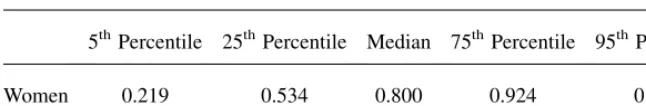
The 1990 PUMS reports three-digit Standard Industrial Classification (SIC) codes and Standard Occupational Classification (SOC) codes for 235 civilian industries and 501 civilian occupations. There are 52,709 observed civilian industry-occupation combinations. The statistic of interest is the fraction of workers between the ages of 18 and 55 who are female in each industry-occupation cell. Distributions of sex-mix statistics for the regression sample are reported in Table 1. The median woman in the regression sample works in an industry-occupation that is 80 percent female, while the median man in the regression sample works in an industry-occupation that is 19 percent female. There is, however, substantial variation in the sex mix experi-enced by men and women on the job. For example, a quarter of women work in occu-pations that are at least 46 percent male, and a quarter of men work in occuoccu-pations that are at least 41 percent female.
To give examples of highly segregated industry-occupation cells, among larger cells with at least 10,000 observations in the PUMS, categories with less than 12 per-cent women include mechanics working in auto repair shops or motor vehicle dealer-ships, many construction occupations (including supervisors, laborers, painters, electricians, and structural metalworkers), landscapers, truck drivers, police officers, and religious clergy. Among the larger cells, categories with at least 92 percent women include preschool teachers, sewing machine operators in the apparel manufacturing industry, cashiers in department stores, hairdressers in beauty shops, secretaries in several industries (including insurance, legal, hospitals and schooling), nurses in hospitals, and nursing aids/attendants in nursing homes.
An examination of the above list of industry-occupation cells emphasizes that the sex mix in industry-occupation cell can only operate as a proxy for actual job-related contact with the opposite sex. Male clergy interact with female parishioners, female hairdressers interact with male clients, and female secretaries in law firms interact with male lawyers. Even so, it is reasonable to believe that there is a real correlation
Table 1
Distribution of Fraction Female in Industry-Occupation
5thPercentile 25thPercentile Median 75thPercentile 95thPercentile
Women 0.219 0.534 0.800 0.924 0.989
Men 0.016 0.059 0.192 0.415 0.750
between the industry-occupation sex mix and true workplace contact. For example, the secretaries in law firms will likely have lunch with the other secretaries, while the lawyers will largely have lunch with the other lawyers.2
Another obvious point from the list above is that occupations and industries vary tremendously in both the quantity and intensity of contact with other people. It would of course be extremely interesting to have data that allowed us to quantify these dif-ferences. We could, for example, test what places you at higher risk for divorce: meeting lots of members of the opposite sex, or having very intensive interactions with a few members of the opposite sex (for example, a police officer and his/her partner). This is, of course, beyond the scope of the current analysis.
B. Sample of Analysis
The sample from the 1990 PUMS used in the regression analysis includes all ever-married, nonwidowed, noninstitutionalized individuals aged 18–55 who report an industry and occupation. Individuals are dropped from the sample if their industry-occupation cell is too small to calculate the sex-mix measure and wage controls used in the regression analysis. Specifically, industry-occupation cells with no more than five observations or without two male workers and two female workers with wages in the range of $2–$200/hour are omitted from the sample. Respondents for whom mar-ital status, industry or occupation are allocated are omitted from the sample. The final sample consists of 1,907,701 women and 1,853,243 men.
One concern about the sample is that only those individuals who have worked within the past five years will report an industry or an occupation in the Census data. Among noninstitutionalized ever-married women aged 18–55 in the 1990 Census, 14.8 percent of married women do not report an industry or occupation and 9.2 per-cent of divorced women similarly must be excluded from the sample. For the sample of men, 1.8 percent of married men and 5.1 percent of divorced men do not report an occupation or industry. The sample used in the analysis conditions on a certain level of labor force attachment, which can be endogenously determined by marital status.
C. OLS Regression Model
The baseline regression model used is the linear probability model:
Yionps=b0+b1FractionFemale_ INDOCCon+WageControls_ INDOCConb2
+b3FractionFemale_ PUMAp+b4ðFractionFemale_ PUMApÞ2
+PUMAControlspb5+IndividualControlsionpsb6+STATEsd
+ðSTATEsUrbaniÞf+eionps; ð1Þ
where for person iin occupationoand industryn, living in Public Use Microdata Area (PUMA)pin states,Yis an indicator for divorce.3Yequals 1 if the respondent
2. Additionally, workplace sex mix likely differs from the sex mix in industry-occupation cell. Because industry-occupation sex mix is an aggregation of workplace sex mix within the industry-occupation cell, the industry-occupation sex mix islessnoisy than the workplace sex mix, and therefore should not generate attenuation bias.
is currently divorced at the time of the 1990 Census.FractionFemale_INDOCCis, for the individual’s industry-occupation cell, the fraction of workers aged 18–55 who are female. To be clear, the fraction female in industry-occupation cell is cal-culated usingall workers aged 18–55, while the regression sample is restricted to ever-married workers.WageControls_INDOCCis a vector of wage controls for the worker’s industry-occupation cell. Specifically, mean male and female wages and the logarithms of male and female wage variances are calculated from the 1990 PUMS for each industry-occupation cell.4 FractionFemale_PUMA is the fraction of residents of the PUMA aged 18–55 who are female.PUMAControlsis a vector of local economic controls that includes the fraction of men employed in the PUMA, the fraction of women employed in the PUMA, the mean male and female wages and the logarithms of male and female wage variances in the PUMA.IndividualControls
is a vector of individual control variables, which includes age, age-squared, race indi-cators (black, Asian, and other), a Hispanic ethnicity indicator, an urban residence indicator, and education indicators (high school degree, some college, college de-gree, and more than college degree).STATEis a vector of state indicator variables andSTATE*Urbaninteracts the state indicators with an indicator for urban residence. These state fixed-effects and state-urban fixed-effects control for unobserved differ-ences across states and differdiffer-ences between urban and rural areas within states. De-scriptive statistics for variables other than the wage controls are reported in Table 2. Descriptive statistics for the wage measures are reported in Appendix 1.
The cross-sectional nature of the data limits the information regarding marital sta-tus. The Census only identifies whether an individual is married, divorced, separated, widowed, or has never married at the time of the survey. If an individual has previously divorced and then remarried, we only observe that person as currently married; we do not know that they were previously divorced. In this paper, those reported as married, divorced, or separated are included in the sample and only those that report they are currently divorced are categorized as such. The analysis with the Census will not cap-ture the effect of workplace contact that generate divorces that are quickly followed by remarriage. But to the extent that workplace contact, through the mechanisms dis-cussed above, generates divorce that is not quickly followed by remarriage, part of the effect of interest can be identified in the cross-sectional census data.5
The census data report current, or most recent, industry and occupation, which could be different from the industry and occupation at the time of divorce. For the purposes of this analysis, changes in industry-occupation cell itself matter less than changes in the industry-occupation sex mix. Calculations of cross-time correlations of fraction female in industry-occupation from the NLSY79 data, which provides longitudinal data on industry and occupation, indicate that the one-year correlation ranges from 0.74 to 0.86 and the five-year correlation ranges from 0.71 to 0.79
4. Individual wages are not included as controls, as these could obviously be endogenous to marital status. The same is true for fertility-related measures.
(variation in correlation is across base-year of observation). Therefore, there is sub-stantial persistence over time in individual’s sex mix in industry-occupation.
D. OLS Regression Results
The initial regression results obtained from Equation 1 are reported in Column 1 of Table 3. Standard errors are clustered at the industry-occupation cell. The negative co-efficient for women is statistically significant, indicating that working in an industry-occupation with a higher fraction of female workers lowers the probability of divorce. The positive coefficient for men indicates that working in an industry-occupation with a higher fraction female raises the probability of divorce, although the result is not statistically significant.
The OLS results suggest stronger effects for women than for men. The effect of sex mix in occupation and industry could differ between men and women for any number of reasons. For example, if the amount and nature of contact with coworkers differs between jobs in male-dominated occupations and jobs in female-dominated occupations, a job that is 75 percent female may not have the same effect on search costs for men as a job that is 75 percent male has on search costs for women.
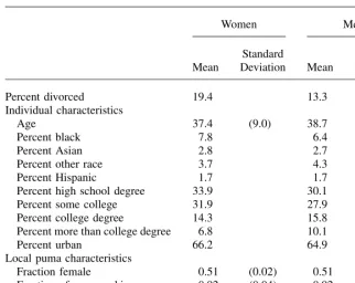
Table 2
Descriptive Statistics, 1990 Census
Women Men
Mean
Standard
Deviation Mean
Standard Deviation
Percent divorced 19.4 13.3
Individual characteristics
Age 37.4 (9.0) 38.7 (8.7)
Percent black 7.8 6.4
Percent Asian 2.8 2.7
Percent other race 3.7 4.3
Percent Hispanic 1.7 1.7
Percent high school degree 33.9 30.1
Percent some college 31.9 27.9
Percent college degree 14.3 15.8
Percent more than college degree 6.8 10.1
Percent urban 66.2 64.9
Local puma characteristics
Fraction female 0.51 (0.02) 0.51 (0.02)
Fraction of men working 0.92 (0.04) 0.92 (0.04)
Fraction of women working 0.78 (0.06) 0.78 (0.06)
N = 1,907,701 N = 1,853,243
Alternatively, if married women in male-dominated occupations are more likely to be approached romantically by their coworkers than married men in female-dominated occupations, this would also generate asymmetric effects. It is not possible with the current data to test among the different explanations for the asymmetric effects.
E. Fixed-Effects Analysis
Choice of occupation and industry is potentially endogenous. One might argue, for example, that women that enter male-dominated occupations are more independent and less family oriented and will be more prone to divorce regardless of exposure to alternative mates.
It should be noted that the selection could work in the opposite direction. Women who work in male-dominated occupations tend to have higher educational attain-ment. Education is negatively correlated with divorce, probably due in part to the fact that these women delay marriage to later ages, which should increase the quality of the match. Therefore, it is also possible that women who work in more sexually in-tegrated occupations have unobserved characteristics that make them less, not more, prone to divorce.
One solution is to include industry and occupation-specific fixed-effects in the model. This will sweep out any unobserved industry and occupation characteristics. For example, if women in more male-dominated occupations work longer hours and have fewer children than women in more traditional occupations, these fixed-effects will purge out mean fertility and mean hours of work by occupation and industry. The model remains identified by the variation at the industry-occupation cell level.
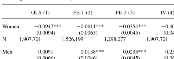
Table 3
Fixed-Effects and IV Estimates, 1990 Census
OLS (1) FE-1 (2) FE-2 (3) IV (4)
Women 20.0947*** 20.0611*** 20.0354*** 20.4019***
(0.0094) (0.0063) (0.0045) (0.0462)
N 1,907,701 1,526,199 1,298,077 1,907,701
Men 0.0091 0.0138*** 0.0295*** 0.2350***
(0.0066) (0.0046) (0.0045) (0.0644)
N 1,853,243 1,482,626 1,203,864 1,853,243
The results of the fixed-effects analysis are reported in Columns 2 and 3 of Table 3. Column 2 reports the results from adding all 501 occupation fixed-effects and all 235 industry fixed-effects to the basic model estimated in Column 1. Standard errors are clustered at the industry-occupation cell. Column 3 reports the results from estimating the fixed-effects model with the sex mix and wage controls for each industry-occupation cell calculated at the state, rather than national, level. In both models, the results for both the men and women are of predicted sign and statistically significant. The effects for men and women are also more similar in magnitude compared to the OLS results. The magnitude of the coefficient on fraction female in industry-occupation cell reported in Column 3 is such that moving a woman from the 25thpercentile to the 75th percentile of fraction female in industry-occupation cell, from 0.534 to 0.924, would decrease her probability of divorce by 1.4 percentage points, or 7.2 percent of the mean female divorce probability of 0.194. The coefficient estimate in Column 3 indicates that moving a man from the 25thpercentile to the 75thpercentile of frac-tion female in industry-occupafrac-tion cell, from 0.059 to 0.415, would increase his probability of divorce by 1.1 percentage points, or 7.9 percent of the mean male di-vorce probability of 0.133.
F. IV Analysis
As an alternative approach to address the endogeneity of occupation and industry choice, the sex mix a worker faces in his or her occupation or industry is instrumented with the industrial and occupational composition of employment in the worker’s local labor market. This instrument varies by sex and by PUMA, but not by industry or occupation. For a male worker in PUMAp, the instrument for the fraction employ-ment in a worker’s occupation that is female is:
IVMaleOCCp=+ o
ShareMaleEmpopFractionFemale_ OCCo; ð2Þ
whereShareMaleEmpopis the fraction of total male employment in PUMA pthat
occurs in occupation oandFractionFemale_ OCCo is the fraction ofnational
em-ployment in occupationothat is female. An analogous instrument can be calculated for the fraction female in a male worker’s industry:
IVMaleINDp=+ n
ShareMaleEmpnpFractionFemale_ INDn; ð3Þ
whereShareMaleEmpnpis the fraction of total male employment in PUMA pthat
occurs in industry nandFractionFemale_ INDn is the fraction of national
employ-ment in industrynthat is female.
The instruments for a female worker in PUMApare:
IVFemOCCp=+ o
ShareFemEmpopFractionFemale_ OCCo; ð4Þ
and:
IVFemINDp=+ n
ShareFemEmpnpFractionFemale_ INDn: ð5Þ
sex-mix measures, where the weights are the shares of local male and female em-ployment in those industries and occupations. Each instrument is therefore an expected value for fraction female in industry or occupation given a worker’s sex and PUMA of residence. Male workers in mining areas in rural Virginia, Kentucky, Nevada, and Texas, for example, are assigned the very lowest values ofIVMaleIND, because they live in areas where a large fraction of men work in mining industries that are overwhelmingly male and are therefore most likely to be working with all men. Male workers in some of the PUMAs in New York City, District of Columbia, Philadelphia, Los Angeles, and San Francisco, where male employment is predomi-nantly in the more integrated industries of real estate, legal services, real estate, and restaurants, receive the highest values of IVMaleIDbecause they are more likely working in very integrated environments.
These examples raise a concern. While these instruments have the appeal that they should be substantially less correlated with individual characteristics than individ-ual’s own choice of occupation and industry, areas that have large shares of employ-ment in integrated industries and occupations may differ in social attitudes from places with large shares of employment in segregated industries and occupations. It should be noted, however, that the regressions control for state fixed-effects and state-urban fixed-effects. Therefore, the effect of interest is not identified from com-paring divorce in rural Kentucky to divorce in New York City. Nor is it identified from comparing rural central Pennsylvania to Philadelphia. The relevant variation in the instruments iswithinurban/rural classificationwithinstate. Unobserved het-erogeneity in PUMA characteristics should therefore be less problematic.
Instrumental variables results are reported in Column 4 of Table 4. The results are of the predicted sign and the effects are larger in magnitude than those obtained with OLS or fixed-effects estimation. These estimates indicate that moving a woman from the 25thpercentile to the 75thpercentile of fraction female in industry-occupation cell decreases her probability of divorce by 15.7 percentage points. Moving a man from the 25thpercentile to the 75thpercentile of fraction female in industry-occupation cell
increases his probability of divorce by 8.4 percentage points. These are very sizeable effects. Unlike the fixed-effects results, but in keeping with the OLS results, these estimates imply a larger effect of sex mix on divorce for women than for men.
IV. NLSY Analysis
members of the couple on divorce. Additional advantages of the NLSY79 are that it, unlike the Census data, provides predivorce information on industry-and occupa-tion, and that it provides a richer set of individual characteristics to use as controls. These advantages come at a cost. The primary disadvantage of the NLSY79 data compared to the 1990 Census is the substantial reduction in sample size. This will limit the potential to use the fixed-effects and instrumental variables strategies employed above to deal with endogenous choice of industry and occupation. An additional dis-advantage is that the NLSY79 is a relatively young sample, with respondents ranging in age from 35 to 42 in 2000, the last year of data used in this analysis.
While the Census data only provided a post-divorce measure of industry-occupation sex mix, the NLSY79 data provides longitudinal information on industry and occupa-tion. This will be exploited in two different methods of analysis. The first will be cross-sectional analysis that uses industry and occupation at the time of marriage. The ad-vantage of this specification is that industry and occupation choices at the beginning of the marriage are plausibly more exogenous to the stability and quality of the marriage than industry and occupational choice in later years, particularly ones that occur right before divorce. The disadvantage of this specification is that it is possible that the sex mix experienced at the time of marriage could be very different from the sex mix ex-perienced years later at the time of divorce. Although, as mentioned earlier, correla-tions calculated from the NLSY sample used in this analysis suggest a very high correlation over time in fraction female in industry-occupation.
Separate hazard-rate analysis will use the longitudinal nature of the data to predict the probability of divorce in a given year based on sex mix in industry-occupation in the same year. In this case, we can be more confident that we are measuring the ac-tual sex mix experienced at the time of divorce, but might be concerned that individ-ual’s adjust their occupational or industry choices as their marriage deteriorates and divorce becomes eminent.
A. OLS Analysis
The analysis sample consists of all ever-married respondents, excluding those in the military oversample, who report the necessary industry and occupation information. Only first marriages are used in the analysis. The respondent’s industry and occupa-tion reported for the year of marriage are used to calculate the respondent’s sex mix in industry-occupation cell. Spouse’s occupation reported for the year of marriage is used to calculate the sex mix in the spouse’s occupation. Spouse’s industry is not reported in the NLSY79 data. For respondents with missing industry or occupation information for the year of marriage, information from most recent job reported in the past five years is used. Because spousal information is not reported prior to the year of marriage, occupation of spouse cannot be filled in from prior information.
The regression model is a linear probability model of the form:
Yiondps=b0+b1FractionFemale_ INDOCCon
+b2FractionFemale_ SpouseOccd+WageControlsondb3
+LocalControlspb4+IndividualControlsib5+STATEsd
where for personiin occupationo and industryn, with a spouse in occupation d, living in local areapin state s,Yis an indicator that equals one if the individual reports ending their first marriage in divorce at any time in the NLSY survey. Frac-tionFemale_INDOCCis, for the respondent’s industry-occupation cell at the time of marriage, the fraction of workers aged 18–40 who are female. FractionFemale_Spouse-Occis, for the spouse’s occupation at the time of marriage, the fraction of workers aged 18–40 who are female.WageControlsis a vector containing mean male and fe-male wages for respondent’s industry-occupation cell and mean fe-male and fefe-male wages for spouse’s occupation, all calculated using workers aged 18–40. For mar-riages in years 1979–85, the sex mix and wage measures are calculated from 1980 Census data. Sex mix and wage measures calculated from 1990 Census data are used for marriages after 1985.
LocalControls includes the local fraction female and local wage and employ-ment measures for the respondent’s county group as calculated from the 1980 Cen-sus for marriages from 1979–1985 and characteristics of the respondent’s PUMA as calculated from the 1990 Census for marriages after 1985. IndividualControls
is a vector of individual control variables, described below.STATE is a vector of state indicator variables andSTATE*Urbaninteracts the state indicators with an in-dicator for urban residence. The local controls, state fixed-effects, and state-urban effects are all based on location at the time of marriage.OCCis a vector of occu-pation fixed-effects,IND is a vector of industry fixed-effects, andSpouseOCC is a vector of spouse occupation fixed-effects, all calculated at the one-digit level. Even though occupation and industry are reported at the three-digit SIC/SOC code level, the smaller sample size of the NLSY79 requires that fixed-effects be limited to the one-digit code level. The full digit-digit codes are used to match in sex mix and wage data. Because the NLSY79 is a stratified sample, the regression is weighted using the initial weights reported for the 1979 survey.
The individual controls used in the OLS analysis are the age of first marriage, race/ethnicity indicators (black, Hispanic), highest grade completed, highest grade completed of spouse, indicator for living with both biological parents at age 14, the respondent’s expected age of marriage (measured in 1979), and expected num-ber of children (measured in 1979).6 Table 4 reports descriptive statistics for the NLSY sample. While a total of 8,553 first marriages are reported in the NLSY79, 3,047 of which end in divorce during the survey, only 5,109 marriages are ob-served with the necessary industry, occupation, and spouse occupation information to be included in the analysis. Approximately one-third of the excluded marriages are missing the necessary occupation and industry information because they occur before 1979, the first year of the survey. Many of the remaining marriages with missing data on industry and occupation are marriages by young respondents, who marry before they ever work. Of the 5,109 marriages with the necessary in-dustry and occupation information, 1,578, or roughly 30 percent, of these mar-riages end in divorce during the survey. The statistics reported in Table 4 indicate that because men tend to marry at later ages than women do, the
marriages reported by male respondents tend to occur slightly later in the survey. As a result, the divorces reported by male respondents tend to occur earlier in the marriage.
Estimates were also obtained using an expanded set of controls. These additional controls included the age difference between the respondent and spouse, indicator for foreign birth, indicator for living in the South at age 14, indicator for urban residence at age 14, indicator for living with a single mom at age 14, mother’s completed years of education, father’s completed years of education, indicator for Protestant upbring-ing, indicator for Catholic upbringupbring-ing, indicator for upbringing in another religion, birth year fixed-effects, interactions of birth year fixed-effects with expected age of marriage, interactions of birth year fixed-effects with expected number of children, and the logarithm of male and female wage variances for industry-occupation cell, spouse’s occupation, and local area. Because adding the additional set of controls de-creased the sample size by 20 percent, the additional controls were rarely statistically significant, and the coefficient estimates on the sex-mix measures changed relatively
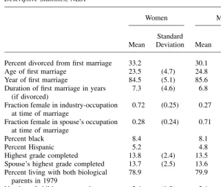
Table 4
Descriptive Statistics, NLSY
Women Men
Mean
Standard
Deviation Mean
Standard Deviation
Percent divorced from first marriage 33.2 30.1
Age of first marriage 23.5 (4.7) 24.8 (4.5)
Year of first marriage 84.5 (5.1) 85.6 (5.0)
Duration of first marriage in years (if divorced)
7.3 (4.6) 6.8 (4.3)
Fraction female in industry-occupation at time of marriage
0.72 (0.25) 0.27 (0.25)
Fraction female in spouse’s occupation at time of marriage
0.28 (0.24) 0.71 (0.25)
Percent black 8.4 8.1
Percent Hispanic 5.2 4.8
Highest grade completed 13.8 (2.4) 13.5 (2.7)
Spouse’s highest grade completed 13.7 (2.5) 13.6 (2.3)
Percent living with both biological parents in 1979
78.9 79.9
Number of children expected (measured 1979)
2.4 (1.3) 2.4 (1.2)
N = 2,736 N = 2,355
little with the additional controls, the results reported here are estimated using the smaller set of controls.
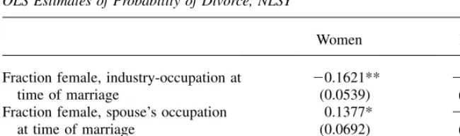
The results obtained from estimating Equation 6 are reported in Table 5. Stan-dard errors are clustered at the industry-occupation level. The results are consistent with expectations. For a married female respondent in the NLSY, working in an industry-occupation with a higher fraction of women lowers her probability of di-vorce. A higher fraction of women in her husband’s occupation increases her prob-ability of divorce. Using the metric of moving from the 25th percentile to the 75th percentile of the sex-mix measure as reported in Table 1, a woman moving from an industry-occupation sex-mix measure of 0.539 to 0.922 would decrease her prob-ability of divorce by 6.2 percentage points. Her husband moving from an occupa-tional sex mix of 0.062 to 0.410 would increase her probability of divorce by 4.8 percentage points.
The results for male respondents are reported in Column 2 of Table 5. The coef-ficient estimates are all small in magnitude, wrong-signed for the man’s own sex mix, and statistically insignificant. It is important to point out that this asymmetry is dif-ferent from that found in the Census analysis. The census results suggested larger effects for women than for men, and this is consistent with the results for the female respondents in Column 1 of Table 5. The woman’s own sex mix has a larger effect on divorce than her husband’s sex mix. In the results for male respondents in Column 2, we would expect to see a positive effect of own fraction female on divorce and a larger, negative effect of the wife’s fraction female on divorce. Instead, we find no evidence of effects for either the man’s sex mix or his wife’s. Some possible explan-ations are discussed further below.
Table 5
OLS Estimates of Probability of Divorce, NLSY
Women Men
Fraction female, industry-occupation at time of marriage
20.1621** 20.0335
(0.0539) (0.0636)
Fraction female, spouse’s occupation at time of marriage
0.1377* 20.0733
(0.0692) (0.0568)
N 2,338 2,034
B. Discrete-Time Hazard Model Analysis
The analysis in this section uses a discrete-time hazard model of the form:
HðtÞ= PrðDivorce in Year tjMarried but Not Divorced in Year t1Þ
=F½b0+b1FractionFemale_ INDOCCont
+b2FractionFemale_ SpouseOccdt+WageControlsondtb3
+LocalControlsptb4+IndividualControlsib5+STATEstd
+ðSTATEstUrbanitÞf+OCCotg1+INDntg2+SpouseOccdtg3+Yeartl
+gðYeart2Year of MarriageiÞ; ð7Þ
for personiworking in occupationoand industryn, living in local areap, in states, in yeart. In this specification, the sex-mix measures are calculated for industry, oc-cupation, and spouse’s occupation at timet. Similarly, wage controls, local controls, state effects, state-urban effects, and industry and occupation code fixed-effects are all measured based on location, industry, occupation, and spouse’s occu-pation at timet. The individual controls are the same as those used in Table 5. Year effects are included in the model and the baseline hazard, g(.) is a vector of dummy variables for duration of marriage, where the hazard is assumed to be constant after ten years of marriage. Assuming thatF[.] is logistic, this specification amounts to estimating logit models where each observation represents a year of marriage for a respondent. Initial 1979 weights are used to weight the regressions.
Using the hazard model expands the sample used for analysis. Individuals who married prior to 1979 can now be included in the analysis, as long as they do not divorce prior to 1979. Individuals who do not report an industry or occupation the year they get married or prior to getting married can now be included in the sample for the years in which industry and occupation are reported. The same is true for cases in which spouse’s occupation is not reported in the initial year of marriage.
If the hazard model is estimated only using observations in which industry, occu-pation, and spouse’s occupation are reported for that year, this will generate a sample that is heavily selected on labor force participation. This is problematic given that labor supply is endogenous to marriage and divorce decisions. Two alternative approaches are used to better deal with nonparticipation. The first is very similar to the occupation and industry measures used in the Census. If occupation, industry or spouse’s occupation is missing in a given year, information from the most recent job reported in the past five years is used. If there is no job information within the past five years, then the observation drops from the sample. This approach produces a sample substantially less selected on labor force attachment. The drawback of this approach is that the sex-mix measures will sometimes reflect the sex mix the respon-dent faced on a job they held many years ago, which if they are not currently work-ing, is less likely to generate a divorce.
measure is set to zero. This is effectively an interaction between an employment in-dicator and the sex mix an individual would experience if they chose to work. The same procedure is used for the sex mix in spouse’s occupation. These two sex-mix measures are then used in the analysis while also controlling for employment of both the respondent and the spouse.7
The results of the hazard model analysis are reported in Table 6. The top panel reports the results obtained using sex mix in most recent job in the past five years. Once again, the results for female respondents conform to expectations. For a female respondent, a higher fraction of female workers in her industry-occupation cell reduces the probability of divorce, while a higher fraction of female workers in her spouse’s occupation increases the probability of divorce. The coefficient for fraction female in industry-occupation is strongly statistically significant, but the co-efficient for fraction female in spouse’s occupation is not significant. For male respondents, the results are similar to those in Table 5; both coefficients are small, negative, and insignificant.
The magnitudes of the effects can be calculated by setting all other controls to their sample means and calculating the effect of the interquartile move on the one-year divorce probability. For a woman with average characteristics, moving from the 25th to 75th percentile of the sex-mix measure decreases her one-year divorce probability from 1.68 percent to 1.28 percent, a decrease of 24 percent. For a woman with average characteristics, moving her husband from the 25thto the 75thpercentile of the sex-mix measure increases her one-year divorce probability from 1.39 to 1.54, an increase of 11 percent.
The bottom panel of Table 6 reports the results from the alternative specification that controls for employment. For the female respondents, own sex mix continues to have a significant negative coefficient, while husband’s sex mix becomes small, neg-ative, and insignificant. The results for male respondents, reported in the second col-umn, continue to be negative and insignificant. The direct labor force participation measures are all insignificant, although of expected sign in the estimates for the fe-male respondents: husband’s work lowers divorce hazard and wife’s work raises it. The lack of agreement between the results for female respondents and the results for male respondents is puzzling. While it is not clear why these differences exist, it is at least possible to discuss some of the differences in the data for male and female respondents that might contribute to this lack of symmetry. One potentially important difference is that because the respondent reports all information for both herself and her spouse, the employment information for both the husband and wife is reported by the wife in the female sample and by the husband in the male sample. Female respondents in the analysis sample used in Table 6 report an employment rate of 77 percent for themselves and 81 percent for their spouses. Male respondents in the same sample report an employment rate of 90 percent for themselves and 63 per-cent for their spouses. This suggests that differences in the accuracy with which men
and women report their own and their spouse’s employment information, including their occupation information, might contribute to the differences in the two sets of results. A second difference between the male and female sample, as shown in Table 4, is that the men typically marry later in the survey so that there are fewer observa-tions on marriage, and fewer marriages of long duration, in the male sample. Finally, because there is relatively little background information on the spouse, the individual controls are largely for the wife in the female sample and are largely for the husband in the male sample.
V. Conclusion
This paper presents evidence that the fraction of workers industry-oc-cupation cell that are female affects the probability an individual is divorced. Women who work with more men are more likely to be divorced and men who work with more women are more likely to be divorced. Most results indicate that the effects are larger for women than for men. It is not possible with the data at hand to
Table 6
Divorce Hazard Results, NLSY
Women Men
Occupation and industry within past five years
Fraction female, industry-occupation 20.7210*** 20.0951
(0.2109) (0.2721)
Fraction female, spouse’s occupation 0.2930 20.1089
(0.2960) (0.2159)
N 32,729 25,887
Occupation and industry for current year’s work
Fraction female, industry-occupation 20.6904*** 20.2378
(0.2160) (0.2804)
Fraction female, spouse’s occupation 20.0478 20.1553
(0.2828) (0.2469)
Worked this year 0.9430 0.6900
(0.4078) (0.4505)
Spouse worked this year 20.1927 0.2009
(0.3040) (0.3809)
N 33,232 26,446
determine whether this is because the predominantly female jobs and the predomi-nantly male jobs differ in their type of workplace contact or whether married men and married women differ in the extent to which they initiate and respond to work-place contact with the opposite sex.
Some of the estimates in this paper are sizeable, leading one to wonder if they are perhaps too big. There are three reasons to believe that a sizable relation does exist. First, if the workplace is now the primary venue for extra-marital search, a substan-tial relationship between occupational sex mix and divorce is perhaps not so surpris-ing. A recent book by psychologist and infidelity expert Shirley Glass, calledNot ‘‘Just Friends,’’proclaims on page one, ‘‘Today’s workplace has become the new danger zone of romantic attraction and opportunity.’’ Second, work by Chiappori and Weiss (2001) discussed above suggests that marriage markets have features that make them highly sensitive to exogenous shocks, such as the infusion of women into the workforce. Finally, the large effects obtained in this analysis are consistent with those found using data on Swedish firms by Aberg (2003).
Appendix 2
Sample for Analysis with Census Data
This appendix contains additional notes on the sample used in Table 3. Dropping industry-occupation cells with five or few workers omits 39,991 individuals, a little less than one percent of the sample. Additionally, only wage observations in the range of $2–$200/hour are used in the calculation of the wage controls. Two workers of each sex with wage observations in this range are necessary to calculate the wage dispersion measures for an industry-occupation cell. Dropping industry-occupation cells without two wage observations for each sex omits another 102,499 workers,
Appendix 1
Summary Statistics for Mean Wage and Wage Dispersion
Women Men
Mean
Standard
Deviation Mean
Standard Deviation
Mean wage, industry-occupation
Male 12.33 (5.00) 14.38 (5.77)
Female 9.29 (3.22) 11.11 (3.71)
Mean wage, occupation
Male 12.51 (4.38) 14.26 (5.21)
Female 9.78 (2.90) 10.79 (3.06)
Mean wage, industry
Male 14.11 (5.23) 13.79 (3.87)
Female 9.73 (2.07) 9.99 (1.75)
Mean wage, PUMA
Male 13.31 (3.03) 13.35 (13.35)
Female 9.60 (1.89) 9.61 (9.61)
Wage variance, industry-occupation
Male 109.99 (159.71) 124.55 (138.58)
Female 66.73 (77.81) 82.39 (143.54)
Wage variance, occupation
Male 110.89 (77.07) 128.31 (117.24)
Female 67.44 (36.43) 81.61 (59.77)
Wage variance, industry
Male 157.75 (134.32) 129.46 (96.35)
Female 70.43 (21.40) 70.32 (21.77)
Wage variance, PUMA
Male 125.28 (72.03) 125.85 (72.96)
Female 68.21 (31.33) 68.39 (31.44)
or another 2.7 percent of the sample. A total of 19,271 industry-occupation cells remain.
Due to computer memory constraints, the results in Column 2 of Table 3 are esti-mated using an 80 percent sample of the 1,907,701 observations available for women and the 1,853,243 observations available for men. Because of the requirement that there be more than five workers to calculate sex mix and wage statistics for industry-occupation cell, calculating these measures at the state level for the analysis in Column 3 reduces the sample by 28 percent to 1,337,791 for men and by 24 percent to 1,442,226 for women. The results in Column 3 are estimated using a 90 percent sample of the 1,442,226 observations available for women and the 1,337,791 obser-vations available for men. Estimating the OLS model used in Column 1 of Table 3 on these reduced samples produces estimates similar to those reported in Column 1.
References
Aberg, Yvonne. 2003. ‘‘Social Interactions: Studies of Contextual Effects and Endogenous Processes.’’ Dissertation. Stockholm: Stockholm University, Department of Sociology. Angrist, Joshua. 2002. ‘‘How do Sex-Ratios Affect Marriage and Labor Markets? Evidence
from America’s Second Generation.’’Quarterly Journal of Economics117(3): 997–1038.
Bayard, Kimberly, Judith Hellerstein, David Neumark, and Kenneth Troske. 2003. ‘‘New Evidence on Sex Segregation and Sex Differences in Wages from Matched Employee-Employer Data.’’Journal of Labor Economics21(4):887–922.
Becker, Gary. 1991.A Treatise on the Family,Enlarged Edition. Cambridge: Harvard University Press.
Becker, Gary, Elisabeth Landes, and Robert Michael. 1977. ‘‘An Economic Analysis of Marital Instability.’’Journal of Political Economy85(6):1141–88.
Brien, Michael. 1997. ‘‘Racial Differences in Marriage and the Role of Marriage Markets.’’
Journal of Human Resources32(4):741–78.
Cherlin, Andrew. 1992.Marriage, Divorce, Remarriage.Revised and enlarged edition. Cambridge: Harvard University Press.
Chiappori, Pierre Andre, and Yoram Weiss. 2001. ‘‘Marriage Contracts and Divorce: an Equilibrium Analysis.’’ Working Paper #5-02, Foerder Institute for Economic Research, Tel Aviv: Tel Aviv University.
Fitzgerald, John. 1991. ‘‘Welfare Durations and the Marriage Market.’’The Journal of Human Resources26(3):545–61.
Glass, Shirley P. 2003.Not ‘‘Just Friends’’: Protect Your Relationship from Infidelity and Heal the Trauma of Betrayal.New York: The Free Press.
Greenstein, Theodore. 1990. ‘‘Marital Disruption and the Employment of Married Women.’’
Journal of Marriage and the Family52(3):657–76.
Kreider, Rose, and Jason Fields. 2001. ‘‘Number, Timing and Duration of Marriages and Divorces: 1996.’’Current Population Reports, P70-80, Washington, D.C.: U.S. Bureau of the Census.
Laumann, Edward, John Gagon, Robert Michael, and Stuart Michaels. 1994.The Social Organization of Sexuality: Sexual Practices in the US.Chicago: The University of Chicago Press.
Lerman, Robert. 1989. ‘‘Employment Opportunities of Young Men and Family Formation.’’
Lichter, Daniel, Felicia LeClere, and Diane McLaughlin. 1991. ‘‘Local Marriage Markets and the Marital Behavior of Black and White Women.’’American Journal of Sociology
96(4):843–67.
Macpherson, David, and Barry Hirsch. 1995. ‘‘Wages and Gender Composition: Why do Women’s Jobs Pay Less?’’Journal of Labor Economics13(3):426–71.
McLanahan, Sara. 1991. ‘‘The Two Faces of Divorce: Women’s and Children’s Interest.’’ In
Macro-Micro Linkages in Sociology, ed. Joan Huber, 193–207. Newbury Park, Calif.: Sage Publications.
Michael, Robert. 1988. ‘‘Why Did the Divorce Rate Double Within a Decade?’’ InResearch in Population Economics, ed. T. Paul Schultz, 367–99. Greenwich, Conn.: JAI Press. Mortensen, Dale. 1988. ‘‘Matching: Finding a Partner for Life or Otherwise.’’American
Journal of Sociology94(supplement): s215–s240.
Norton, Arthur, and Louisa Miller. 1992. ‘‘Marriage, Divorce, and Remarriage in the 1990’s.’’
Current Population Reports, P23-180, Washington, D.C.: U.S. Bureau of the Census. Olsen, Randall, and George Farkas. 1990. ‘‘The Effect of Economic Opportunity and Family
Background on Adolescent Cohabitation and Childbearing among Low-Income Blacks.’’
Journal of Labor Economics8(3):341–62.
Ross, Heather, and Isabel Sawhill. 1975.Time of Transition: The Growth of Families Headed by Women.Washington, D.C.: Urban Institute.
Ruggles, Steven. 1997. ‘‘The Rise of Divorce and Separation in the United States, 1880–1990.’’Demography34(4):455–66.
Sorensen, Elaine. 990. ‘‘The Crowding Hypothesis and Comparable Worth.’’The Journal of Human Resources25(1):55–89.
South, Scott. 2001. ‘‘Time-Dependent Effects of Wives’ Employment on Marital Dissolution.’’American Sociological Review66(2):226–45.
South, Scott, and Kim Lloyd. 1995. ‘‘Spousal Alternatives and Marital Dissolution.’’
American Sociological Review60(1):21–35.
South, Scott, Katherine Trent, and Yang Shen. 2001. ‘‘Changing Partners: Toward a Macrostructural-Opportunity Theory of Marital Dissolution.’’Journal of Marriage and the Family63(3):743–54.
Udry, J. Richard. 1981. ‘‘Marital Alternatives and Marital Disruption.’’Journal of Marriage and the Family43(4):889–97.
White, Lynn, and Alan Booth. 1991. ‘‘Divorce over the Life Course: The Role of Marital Happiness.’’Journal of Family Issues12(1):5–21.