El e c t ro n ic
Jo ur
n a l o
f P
r o
b a b il i t y
Vol. 14 (2009), Paper no. 5, pages 87–118. Journal URL
http://www.math.washington.edu/~ejpecp/
On percolation in random graphs with given vertex
degrees
Svante Janson
Department of Mathematics
Uppsala University
PO Box 480
SE-751 06 Uppsala
Sweden
[email protected]
http://www.math.uu.se/~svante/
Abstract
We study the random graph obtained by random deletion of vertices or edges from a random graph with given vertex degrees. A simple trick of exploding vertices instead of deleting them, enables us to derive results from known results for random graphs with given vertex degrees. This is used to study existence of giant component and existence ofk-core. As a variation of the latter, we study also bootstrap percolation in random regular graphs.
We obtain both simple new proofs of known results and new results. An interesting feature is that for some degree sequences, there are several or even infinitely many phase transitions for thek-core.
Key words:random graph, giant component, k-core, bootstrap percolation. AMS 2000 Subject Classification:Primary 60C05; 05C80.
1
Introduction
One popular and important type of random graph is given by the uniformly distributed random graph with a given degree sequence, defined as follows. Letn∈Nand letd= (di)n1be a sequence of non-negative integers. We letG(n,d)be a random graph with degree sequenced, uniformly chosen among all possibilities (tacitly assuming that there is any such graph at all; in particular,Pidi has to be even).
It is well-known that it is often simpler to study the corresponding random multigraphG∗(n,d)with given degree sequenced= (di)1n, defined for every sequencedwithPidi even by the configuration model (see e.g. Bollobás [3]): take a set of di half-edges for each vertex i, and combine the half-edges into pairs by a uniformly random matching of the set of all half-half-edges (this pairing is called a
configuration); each pair of half-edges is then joined to form an edge ofG∗(n,d).
We consider asymptotics as the numbers of vertices tend to infinity, and thus we assume throughout the paper that we are given, for each n, a sequence d(n) = (di(n))1n withPidi(n) even. (As usual, we could somewhat more generally assume that we are given a sequencenν → ∞ and for eachν
a sequenced(ν)= (di(ν))nν
1 .) For notational simplicity we will usually not show the dependency on
n explicitly; we thus writed and di, and similarly for other (deterministic or random) quantities introduced below. All unspecified limits and other asymptotic statements are for n → ∞. For example, w.h.p. (with high probability) means ’with probability tending to 1 as n→ ∞’, and −→p means ’convergence in probability as n→ ∞’. Similarly, we use op and Op in the standard way, always implyingn→ ∞. For example, ifX is a parameter of the random graph, X = op(n)means thatP(X > ǫn)→0 asn→ ∞for everyǫ >0; equivalently,X/n−→p 0.
We may obtainG(n,d)by conditioning the multigraph G∗(n,d)on being a (simple) graph, i.e., on not having any multiple edges or loops. By Janson[9](with earlier partial results by many authors),
lim infP G∗(n,d)is simple>0 ⇐⇒
n X
i=1
di2=O
n X
i=1
di
!
. (1.1)
In this case, many results transfer immediately fromG∗(n,d)toG(n,d), for example, every result of the typeP(En)→0 for some eventsEn, and thus every result saying that some parameter converges
in probability to some non-random value. This includes every result in the present paper.
We will in this paper study the random multigraph G∗(n,d); the reader can think of doing this either for its own sake or as a tool for studying G(n,d). We leave the statement of corollaries for
G(n,d), using (1.1), to the reader. Moreover, the results for G(n,d)extend to some other random graph models too, in particular G(n,p) withp ∼λ/nand G(n,m) withm∼λn/2 withλ >0, by the standard device of conditioning on the degree sequence; again we omit the details and refer to [10; 11; 12]where this method is used.
We will consider percolation of these random (multi)graphs, where we first generate a random graphG∗(n,d)and then delete either vertices or edges at random. (From now on, we simply write ’graph’ for ’multigraph’.) The methods below can be combined to treat the case of random deletion of both vertices and edges, which is studied by other methods in e.g. Britton, Janson and Martin-Löf [4], but we leave this to the reader.
Site percolation Randomly delete each vertex (together with all incident edges) with probability 1−π, independently of all other vertices. We denote the resulting random graph byGπ,v.
Bond percolation Randomly delete each edge with probability 1−π, independently of all other edges. (All vertices are left.) We denote the resulting random graph byGπ,e.
Thus π denotes the probability to be kept in the percolation model. When, as in our case, the original graph G itself is random, it is further assumed that we first sampleG and then proceed as above, conditionally onG.
The casesπ=0, 1 are trivial:G1,v=G1,e=G, whileG0,v=;, the null graph with no vertices and no edges, andG0,eis the empty graph with the same vertex set asG but no edges. We will thus mainly consider 0< π <1.
We may generalize the site percolation model by letting the probability depend on the degree of the vertex. Thus, ifπ= (πd)∞
0 is a given sequence of probabilitiesπd ∈[0, 1], letGπ,v be the random graph obtained by deleting vertices independently of each other, with vertex v ∈ G deleted with probability 1−πd(v)where d(v)is the degree ofvinG.
For simplicity and in order to concentrate on the main ideas, we will in this paper consider only the case when the probabilityπ(or the sequenceπ) is fixed and thus does not depend onn, with the
exception of a few remarks where we briefly indicate how the method can be used also for a more detailed study of thresholds.
The present paper is inspired by Fountoulakis[7], and we follow his idea of deriving results for the percolation modelsG∗(n,d)π,vandG∗(n,d)π,efrom results for the modelG∗(n,d)without deletions, but for different degree sequences d. We will, however, use another method to do this, which we find simpler.
Fountoulakis [7] shows that for both site and bond percolation on G∗(n,d), if we condition the resulting random graph on its degree sequenced′, and let n′be the number of its vertices, then the graph has the distribution ofG∗(n′,d′), the random graph with this degree sequence constructed by the configuration model. He then proceeds to calculate the distributions of the degree sequenced′
for the two percolation models and finally applies known results toG∗(n′,d′).
Our method is a version of this, where we do the deletions in two steps. For site percolation, instead of deleting a vertex, let us first explode it by replacing it by d new vertices of degree 1, where d
is its degree; we further colour the new vertices red. Then clean up by removing all red vertices. Note that the (random) explosions change the number of vertices, but not the number of half-edges. Moreover, given the set of explosions, there is a one-to-one correspondence between configurations before and after the explosions, and thus, if we condition on the new degree sequence, the exploded graph is still described by the configuration model. Furthermore, by symmetry, when removing the red vertices, all vertices of degree 1 are equivalent, so we may just as well remove the right number of vertices of degree 1, but choose them uniformly at random. Hence, we can obtainG∗(n,d)π,v as follows:
Site percolation For each vertexi, replace it with probability 1−πbydi new vertices of degree 1 (independently of all other vertices). Let ˜dπ,vbe the resulting (random) degree sequence, let ˜
nbe its length (the number of vertices), and let n+ be the number of new vertices. Construct
the random graphG∗(˜n, ˜dπ,v). Finish by deletingn+randomly chosen vertices of degree 1. The more general case when we are given a sequenceπ= (πd)∞
Site percolation, general For each vertex i, replace it with probability 1−πdi by di new vertices of degree 1. Let ˜dπ,v be the resulting (random) degree sequence, let ˜n be its length (the number of vertices), and letn+be the number of new vertices. Construct the random graph
G∗(˜n, ˜dπ,v). Finish by deletingn+randomly chosen vertices of degree 1.
Remark 1.1. We have here assumed that vertices are deleted at random, independently of each other. This is not essential for our method, which may be further extended to the case when we remove a set of vertices determined by any random procedure that is independent of the edges in
G(n,d)(but may depend on the vertex degrees). For example, we may remove a fixed numbermof vertices, chosen uniformly at random. It is easily seen that ifm/n→π, the results of Subsection 2.1 below still hold (with all πj = π), and thus the results of the later sections hold too. Another, deterministic, example is to remove the firstmvertices.
For bond percolation, we instead explode each half-edge with probability 1−pπ, independently of all other half-edges; to explode a half-edge means that we disconnect it from its vertex and transfer it to a new, red vertex of degree 1. Again this does not change the number of half-edges, and there is a one-to-one correspondence between configurations before and after the explosions. We finish by removing all red vertices and their incident edges. Since an edge consists of two half-edges, and each survives with probabilitypπ, this gives the bond percolation model G∗(n,d)π,e where edges are kept with probabilityπ. This yields the following recipe:
Bond percolation Replace the degrees di in the sequenced by independent random degrees ˜di ∼
Bi(di,pπ). (I.e., ˜di has the binomial distribution Bi(di,pπ).) Add n+:=
Pn
i=1(di−d˜i)new degrees 1 to the sequence(d˜i)n1, and let ˜dπ,ebe the resulting degree sequence and ˜n=n+n+ its length. Construct the random graph G∗(n˜, ˜dπ,e). Finish by deleting n+ randomly chosen vertices of degree 1.
In both cases, we have reduced the problem to a simple (random) modification of the degree se-quence, plus a random removal of a set of vertices of degree 1. The latter is often more or less trivial to handle, see the applications below. We continue to call the removed vertices red when convenient.
Of course, to use this method, it is essential to find the degree sequence ˜dafter the explosions. We study this in Section 2. We then apply this method to three different problems:
Existence of a giant component in the percolated graph, i.e., what is called percolation in random graph theory (Section 3). Our results include and extend earlier work by Fountoulakis[7], which inspired the present study, and some of the results by Britton, Janson and Martin-Löf[4].
Existence of a k-corein the percolated graph (Section 4). We obtain a general result analogous to (and extending) the well-known result by Pittel, Spencer and Wormald[17]forG(n,p). We study the phase transitions that may occur in some detail and show by examples that it is possible to have several, and even an infinite number of, different phase transitions as the probabilityπ increases from 0 to 1.
Bootstrap percolation in random regular graphs (Section 5), where we obtain a new and simpler proof of results by Balogh and Pittel[1].
For a graphG, let v(G)ande(G)denote the numbers of vertices and edges in G, respectively, and letvj(G)be the number of vertices of degree j, j≥0. We sometimes useG∗(n,d)π to denote any of
2
The degree sequence after explosions
Letnj :=#{i≤n:di = j}. Thus P∞
j=0nj=n, andnj equals the numbervj(G∗(n,d))of vertices of degree j inG∗(n,d). We assume for simplicity the following regularity condition.
Condition 2.1. There exists a probability distribution (pj)∞j=0 with finite positive mean λ :=
P
j j pj∈(0,∞)such that (asn→ ∞)
nj/n→pj, j≥0, (2.1)
and P
∞ j=0jnj
n →λ:=
∞ X
j=0
j pj. (2.2)
Note that, in order to avoid trivialities, we assume thatλ >0, which is equivalent top0<1. Thus,
there is a positive fraction of vertices of degree at least 1.
Note thatPj jnj=Pidi equals twice the number of edges inG∗(n,d), and that (2.2) says that the average degree inG∗(n,d)converges toλ.
Let the random variable Dˆ = ˆDn be the degree of a random vertex in G∗(n,d), thus Dˆn has the distributionP( ˆDn = j) =nj/n, and letD be a random variable with the distribution(pj)∞0 . Then
(2.1) is equivalent to Dˆn −→d D, and (2.2) is EDˆn → λ = ED. Further, assuming (2.1), (2.2)
is equivalent to uniform integrability of Dˆn, or equivalently uniform summability (as n→ ∞) of P
j jnj/n, see for example Gut[8], Theorem 5.5.9 and Remark 5.5.4.
Remark 2.2. The uniform summability ofPj jnj/nis easily seen to imply that ifH is any (random or deterministic) subgraph on G∗(n,d) with v(H) = o(n), then e(H) = o(n), and similarly with
op(n).
We will also use the probability generating function of the asymptotic degree distributionD:
gD(x):=ExD= ∞ X
j=0
pjxj, (2.3)
defined at least for|x| ≤1.
We perform either site or bond percolation as in Section 1, by the explosion method described there, and let ˜nj:=#{i≤n˜: ˜di= j}be the number of vertices of degree jafter the explosions. Thus
∞ X
j=0
˜
nj=n˜. (2.4)
2.1
Site percolation
We treat the general version with a sequenceπ. Let n◦
j be the number of vertices of degree j that are not exploded. Then uniform summability ofPjjnj/n(which enables us to treat the infinite sums in (2.10) and (2.13) by a standard argument),
Hence Condition 2.1 holds, in probability, for the random degree sequence ˜dtoo. Further, the total number of half-edges is not changed by the explosions, and thus also, by (2.14) and (2.2),
hence (or by (2.15)),
˜
λ=ζ−1λ. (2.18)
In the proofs below it will be convenient to assume that (2.15) and (2.16) hold a.s., and not just in probability, so that Condition 2.1 a.s. holds for ˜d; we can assume this without loss of generality by the Skorohod coupling theorem[13, Theorem 4.30]. (Alternatively, one can argue by selecting suitable subsequences.)
Let ˜Dhave the probability distribution(˜pj), and let gD˜ be its probability generating function. Then,
by (2.15),
For bond percolation, we have explosions that do not destroy the vertices, but they may reduce their degrees. Let ˜nl jbe the number of vertices that had degreel before the explosions and jafter. Thus ˜
nj =Pl≥jn˜l j for j6=1 and ˜n1=Pl≥1n˜l1+n+. A vertex of degreel will after the explosions have a degree with the binomial distribution Bi(l,π1/2), and thus the probability that it will become a vertex of degree jis the binomial probability bl j(π1/2), where we define
Since explosions at different vertices occur independently, this means that, forl≥ j≥0, ˜
nl j∼Bi nl,bl j(π1/2)
and thus, by the law of large numbers and (2.1), ˜
nl j=bl j(π1/2)pln+op(n).
Further, the numbern+of new vertices equals the number of explosions, and thus has the binomial
˜
n=n+n+=n+ 1−π1/2λn+op(n). (2.25)
In analogy with site percolation we thus have, by (2.25), ˜
n n
p
−→ζ:=1+ 1−π1/2λ (2.26)
and further, by (2.23) and (2.24),
˜
nj
˜
n
p
−→˜pj:=
ζ−1Pl≥jbl j(π1/2)pl, j6=1, ζ−1P
l≥1bl1(π1/2)pl+ 1−π1/2
λ, j=1. (2.27)
Again, the uniform summability of jnj/nimplies uniform summability of jn˜j/˜n, and the total num-ber of half-edges is not changed; thus (2.16), (2.17) and (2.18) hold, now withζgiven by (2.26). Hence Condition 2.1 holds in probability for the degree sequences ˜d in bond percolation too, and by the Skorohod coupling theorem we may assume that it holds a.s.
The formula for ˜pj is a bit complicated, but there is a simple formula for the probability generating function gD˜. We have, by the binomial theorem,
P
j≤lbl j(π)xj = (1−π+πx)l, and thus (2.27) yields
ζgD˜(x) =
∞ X
l=0
(1−π1/2+π1/2x)lpl+ (1−π1/2)λx
=gD(1−π1/2+π1/2x) + (1−π1/2)λx.
(2.28)
3
Giant component
The question of existence of a giant component inG(n,d)andG∗(n,d)was answered by Molloy and Reed[16], who showed that (under some weak technical assumptions) a giant component exists w.h.p. if and only if (in the notation above) ED(D−2)>0. (The term giant componentis in this paper used, somewhat informally, for a component containing at least a fractionǫ of all vertices, for some smallǫ >0 that does not depend onn.) They further gave a formula for the size of this giant component in Molloy and Reed[15]. We will use the following version of their result, given by Janson and Luczak[12], Theorem 2.3 and Remark 2.6. Let, for any graphG,Ck(G)denote thek:th largest component ofG. (Break ties by any rule. If there are fewer that kcomponents, letCk:=;, the null graph.)
Theorem 3.1 ([15; 12]). Consider G∗(n,d), assuming that Condition 2.1 holds and p1 > 0. Let
Ck:=Ck(G∗(n,d))and let gD(x)be the probability generating function in(2.3). (i) If ED(D−2) =P
j j(j−2)pj>0, then there is a uniqueξ∈(0, 1)such that g′D(ξ) =λξ, and
v(C1)/n−→p 1−gD(ξ)>0, (3.1)
vj(C1)/n−→p pj(1−ξj), for every j≥0, (3.2)
e(C1)/n−→p 21λ(1−ξ2). (3.3)
(ii) If ED(D−2) =Pj j(j−2)pj≤0, then v(C1)/n−→p 0and e(C1)/n−→p 0. Remark 3.2. ED2=∞is allowed in Theorem 3.1(i).
Remark 3.3. In Theorem 3.1(ii), whereED(D−2)≤0 andp1>0, for 0≤x <1
λx−gD′(x) =
∞ X
j=1
j pj(x−xj−1) =p1(x−1) +x
∞ X
j=2
j pj(1−xj−2)
≤p1(x−1) +x
∞ X
j=2
j pj(j−2)(1−x)
<
∞ X
j=1
j(j−2)pjx(1−x) =ED(D−2)x(1−x)≤0.
Hence, in this case the only solution in [0, 1]to g′D(ξ) = λξisξ=1, which we may take as the definition in this case.
Remark 3.4. Let D∗be a random variable with the distribution
P(D∗= j) = (j+1)P(D= j+1)/λ, j≥0;
this is the size-biased distribution ofDshifted by 1, and it has a well-known natural interpretation as follows. Pick a random half-edge; then the number of remaining half-edges at its endpoint has asymptotically the distribution of D∗. Therefore, the natural (Galton–Watson) branching process approximation of the exploration of the successive neighbourhoods of a given vertex is the branching processX with offspring distributed asD∗, but starting with an initial distribution given byD. Since
gD∗(x) =
∞ X
j=1
P(D∗= j−1)xj−1=
∞ X
j=1
j pj λ x
j−1= g′D(x) λ ,
the equation g′D(ξ) =λξin Theorem 3.1(i) can be written gD∗(ξ) =ξ, which shows thatξhas an
interpretation as the extinction probability of the branching processX with offspring distribution
D∗, now starting with a single individual. (This also agrees with the definition in Remark 3.3 for the case Theorem 3.1(ii).) ThusgD(ξ)in (3.1) is the extinction probability ofX. Note also that
ED∗= ED(D−1)
λ =
ED(D−1)
ED ,
so the conditionED(D−2)>0, or equivalentlyED(D−1)>ED, is equivalent to ED∗ >1, the classical condition for the branching process to be supercritical and thus have a positive survival probability.
The intuition behind the branching process approximation of the local structure of a random graph at a given vertex is that an infinite approximating branching process corresponds to the vertex being in a giant component. This intuition agrees also with the formulas (3.2) and (3.3), which reflect the fact that a vertex of degree j [an edge]belongs to the giant component if and only if one of its j
Consider one of our percolation modelsG∗(n,d)π, and construct it using explosions and an inter-mediate random graphG∗(n˜, ˜d)as described in the introduction. (Recall that ˜d is random, whiled
and the limiting probabilities pj and ˜pj are not.) LetCj :=Cj G∗(n,d)π
and ˜Cj:=Cj G∗(n˜, ˜d)
denote the components ofG∗(n,d)π, andG∗(n˜, ˜d), respectively.
As remarked in Section 2, we may assume thatG∗(n˜, ˜d)too satisfies Condition 2.1, with pj replaced by ˜pj. (At least a.s.; recall that ˜d is random.) Hence, assuming ˜p1 > 0, if we first condition on ˜
d, then Theorem 3.1 applies immediately to the exploded graph G∗(n˜, ˜d). We also have to remove
n+ randomly chosen “red” vertices of degree 1, but luckily this will not break up any component.
Consequently, ifED(˜ D˜−2)>0, thenG∗(˜n, ˜d)w.h.p. has a giant component ˜C1, with v(C˜1), vj(C˜1)
and e(C˜1) given by Theorem 3.1 (with pj replaced by ˜pj), and after removing the red vertices, the remainder of ˜C1 is still connected and forms a componentC in G∗(n,d)π. Furthermore, since
ED(˜ D˜ −2) > 0, ˜pj > 0 for at least one j > 2, and it follows by (3.2) that ˜C1 contains cn+ op(n) vertices of degree j, for some c >0; all these belong to C (although possibly with smaller degrees), soC contains w.h.p. at leastcn/2 vertices. Moreover, all other components of G∗(n,d)π
are contained in components ofG∗(˜n, ˜d)different from ˜C1, and thus at most as large as ˜C2, which by
Theorem 3.1 hasop(n) =˜ op(n)vertices. Hence, w.h.p.C is the largest componentC1ofG∗(n,d)π, and this is the unique giant component inG∗(n,d)π.
Since we remove a fractionn+/˜n1of all vertices of degree 1, we remove by the law of large numbers
(for a hypergeometric distribution) about the same fraction of the vertices of degree 1 in the giant component ˜C1. More precisely, by (3.2), ˜C1 contains about a fraction 1−ξof all vertices of degree 1, whereg′˜
D(ξ) =λξ; hence the number of red vertices removed from ˜˜ C1is
(1−ξ)n++op(n). (3.4)
By (3.1) and (3.4),
v(C1) =v(C˜1)−(1−ξ)n++op(n) =n˜ 1−gD˜(ξ)
−n++n+ξ+op(n). (3.5) Similarly, by (3.3) and (3.4), since each red vertex that is removed fromC1 also removes one edge with it,
e(C1) =e(C˜1)−(1−ξ)n++op(n) = 21λ˜˜n(1−ξ2)−(1−ξ)n++op(n). (3.6) The case ED(˜ D˜ −2) ≤ 0 is even simpler; since the largest component C1 is contained in some
component ˜CjofG∗(n˜, ˜d), it follows thatv(C1)≤v(C˜j)≤v(C˜1) =op(n) =˜ op(n).
This leads to the following results, where we treat site and bond percolation separately and add formulas for the asymptotic size ofC1.
Theorem 3.5. Consider the site percolation model G∗(n,d)π,v, and suppose that Condition 2.1 holds
and thatπ= (πd)∞
0 with0≤πd ≤1; suppose further that there exists j ≥1such that pj >0and πj <1. Then there is w.h.p. a giant component if and only if
∞ X
j=0
j(j−1)πjpj> λ:= ∞ X
j=0
j pj. (3.7)
(i) If (3.7)holds, then there is a uniqueξ=ξv(π)∈(0, 1)such that ∞
X
j=1
and then It remains only to verify the formulas (3.8)–(3.10). The equationg′˜
D(ξ) =λξ˜ is by (2.18) equivalent toζg′˜
D(ξ) =λξ, which can be written as (3.8) by (2.15) and a simple calculation. By (3.5), using (2.10), (2.14) and (2.19),
v(C1)/n−→p ζ−ζgD˜(ξ)−(1−ξ)
Similarly, by (3.6), (2.18), (2.14) and (2.10),
e(C1)/n−→p 12λ(1−ξ2)−(1−ξ)
Corollary 3.6([4; 7]). Suppose that Condition 2.1 holds and0< π <1. Then there exists w.h.p. a giant component in G∗(n,d)π,vif and only if
π > πc:= ED
ED(D−1). (3.11)
Remark 3.7. Note that πc= 0 is possible; this happens if and only ifED2 = ∞. (Recall that we
assume 0<ED<∞, see Condition 2.1.) Further,πc≥1 is possible too: in this case there is w.h.p. no giant component in G∗(n,d) (except possibly in the special case when pj =0 for all j 6=0, 2), and consequently none in the subgraphG∗(n,d)π.
Note that by (3.11), πc ∈ (0, 1) if and only if ED < ED(D−1) < ∞, i.e., if and only if 0 < ED(D−2)<∞.
Remark 3.8. Another case treated in[4](there calledE1) is πd =αd for some α∈(0, 1). Theo-rem 3.5 gives a new proof that then there is a giant component if and only ifP∞j=1j(j−1)αjpj> λ, which also can be writtenα2g′′
D(α)> λ=g′D(1). (The casesE2andAin[4]are more complicated and do not follow from the results in the present paper.)
For edge percolation we similarly have the following; this too has been shown by Britton, Janson and Martin-Löf[4]and Fountoulakis[7]. Note that the percolation thresholdπis the same for site and bond percolation, as observed by Fountoulakis[7].
Theorem 3.9 ([4; 7]). Consider the bond percolation model G∗(n,d)π,e, and suppose that
Condi-tion 2.1 holds and that0< π <1. Then there is w.h.p. a giant component if and only if
π > πc:= ED
ED(D−1). (3.12)
(i) If (3.12)holds, then there is a uniqueξ=ξe(π)∈(0, 1)such that
π1/2g′D 1−π1/2+π1/2ξ+ (1−π1/2)λ=λξ, (3.13)
and then
v(C1)/n−→p χe(π):=1−gD 1−π1/2+π1/2ξ>0, (3.14)
e(C1)/n−→p µe(π):=π1/2(1−ξ)λ−12λ(1−ξ)2. (3.15)
Furthermore, v(C2)/n−→p 0and e(C2)/n−→p 0.
(ii) If (3.12)does not hold, then v(C1)/n−→p 0and e(C1)/n−→p 0.
Proof. We argue as in the proof of Theorem 3.5, noting that ˜p1>0 by (2.27). By (2.28),
ζED(˜ D˜−2) =ζg′′
˜
D(1)−ζg ′
˜
D(1) =πg ′′
D(1)−π
1/2g′
D(1)−(1−π
1/2)λ
=πED(D−1)−λ,
which yields the criterion (3.12). Further, if (3.12) holds, then the equation g′˜D(ξ) =λξ, which by˜ (2.18) is equivalent toζg′˜
By (3.5), (2.26), (2.22) and (2.28),
v(C1)/n−→p ζ−ζg˜D(ξ)−(1−ξ)(1−π1/2)λ=1−gD 1−π1/2+π1/2ξ)
, which is (3.14). Similarly, (3.6), (2.26), (2.18) and (2.22) yield
e(C1)/n−→p 12λ(1−ξ2)−(1−ξ)(1−π1/2)λ=π1/2(1−ξ)λ−12λ(1−ξ)2, which is (3.15). The rest is as above.
Remark 3.10. It may come as a surprise that we have the same criterion (3.11) and (3.12) for site and bond percolation, since the proofs above arrive at this equation in somewhat different ways. However, remember that all results here are consistent with the standard branching process approximation in Remark 3.4 (even if our proofs use different arguments) and it is obvious that both site and bond percolation affect the mean number of offspring in the branching process in the same way, namely by multiplication byπ. Cf.[4], where the proofs are based on such branching process approximations.
Define
ρv=ρv(π):=1−ξv(π) and ρe=ρe(π):=1−ξe(π); (3.16)
recall from Remark 3.4 thatξvandξeare the extinction probabilities in the two branching processes defined by the site and bond percolation models, and thusρvandρeare the corresponding survival probabilities. For bond percolation, (3.13)–(3.15) can be written in the somewhat simpler forms
π1/2g′D 1−π1/2ρe=λ(π1/2−ρe), (3.17)
v(C1)/n−→p χe(π):=1−gD 1−π1/2ρe(π), (3.18)
e(C1)/n−→p µe(π):=π1/2λρe(π)−1
2λρe(π)
2. (3.19)
Note further that if we consider site percolation with allπj=π, (3.8) can be written
π λ−g′D(1−ρv)=λρv (3.20)
and it follows by comparison with (3.17) that
ρv(π) =π1/2ρe(π). (3.21)
Furthermore, (3.9), (3.10), (3.18) and (3.19) now yield
χv(π) =π 1−gD(ξv(π))=π 1−gD(1−ρv(π))=πχe(π), (3.22) µv(π) =πλρv(π)−12λρv(π)2=πµe(π). (3.23) We next consider how the various parameters above depend on π, for both site percolation and bond percolation, where for site percolation we in the remainder of this section consider only the case when allπj=π.
Theorem 3.11. Assume Condition 2.1. The functionsξv,ρv,χv,µv,ξe,ρe,χe,µeare continuous func-tions ofπ∈(0, 1)and are analytic except atπ=πc. (Hence, the functions are analytic in(0, 1)if and only ifπc=0orπc≥1.)
Proof. It suffices to show this forξv; the result for the other functions then follows by (3.16) and (3.21)–(3.23). Since the case π ≤ πc is trivial, it suffices to consider π ≥ πc, and we may thus assume that 0≤πc<1.
Ifπ∈(πc, 1), then, as shown above,g′˜
D(ξv) =λξv, or, equivalently,˜ G(ξv,π) =0, whereG(ξ,π):=
g′˜
D(ξ)/ξ−λ˜is an analytic function of(ξ,π)∈(0, 1)
2. Moreover,G(ξ,π)is a strictly convex function
ofξ∈(0, 1]for any π∈(0, 1), and G(ξv,π) = G(1,π) =0; hence ∂G∂ ξ(ξ,π)¯¯ξ=ξ
v
<0. The implicit function theorem now shows thatξv(π)is analytic forπ∈(πc, 1).
For continuity atπc, supposeπc∈(0, 1)and let ξˆ=limn→∞ξv(πn)for some sequence πn →πc. Then, writing ˜D(π)and ˜λ(π)to show the dependence onπ,g′˜
D(πn)
(ξv(πn)) =λ˜(πn)ξv(πn)and thus by continuity, e.g. using (2.28),g′˜
D(πc)
( ˆξ) =λ˜(πc) ˆξ. However, forπ≤πc, we haveED(˜ D˜−2)≤0
and thenξ=1 is the only solution in(0, 1]ofg′˜
D(ξ) =λξ; hence˜ ξˆ=1. This shows thatξv(π)→1 asπ→πc, i.e.,ξvis continuous atπc.
Remark 3.12. Alternatively, the continuity ofξv in(0, 1) follows by Remark 3.4 and continuity of the extinction probability as the offspring distribution varies, cf.[4, Lemma 4.1]. Furthermore, by the same arguments, the parameters are continuous also at π = 0 and, except in the case when
p0+p2=1 (and thus ˜D=1 a.s.), atπ=1 too.
At the thresholdπc, we have linear growth of the size of the giant component for (slightly) larger π, providedED3<∞, and thus a jump discontinuity in the derivative ofξv,χv, . . . . More precisely,
the following holds. We are here only interested in the case 0< πc < 1, which is equivalent to 0<ED(D−2)<∞, see Remark 3.7.
Theorem 3.13. Suppose that0<ED(D−2)<∞; thus0< πc<1. If furtherED3 <∞, then as
ǫց0,
ρv(πc+ǫ)∼ 2ED(D−1)
πcED(D−1)(D−2)ǫ=
2 ED(D−1)2
ED·ED(D−1)(D−2)ǫ (3.24)
χv(πc+ǫ)∼µv(πc+ǫ)∼πcλρv(πc+ǫ)∼ 2ED·ED(D−1)
ED(D−1)(D−2)ǫ. (3.25) Similar results forρe,χe,µefollow by(3.21)–(3.23).
Proof. Forπ=πc+ǫցπc, by gD′′(1) =ED(D−1) =λ/πc, see (3.11), and (3.20),
ǫg′′D(1)ρv= (π−πc)g′′D(1)ρv=πg′′D(1)ρv−λρv=π g′′D(1)ρv−λ+g′D(1−ρv). (3.26) Since ED3 < ∞, gD is three times continuously differentiable on [0, 1], and a Taylor expansion
yields gD′(1−ρv) =λ−ρvgD′′(1) +ρv2g
′′′
D(1)/2+o(ρ
2
Thus, noting that g′′D(1) =ED(D−1)andg′′′
D(1) =ED(D−1)(D−2)>0 (sinceED(D−2)>0),
ρv∼ 2g ′′ D(1) πcg′′′D(1)ǫ=
2ED(D−1)
πcED(D−1)(D−2)ǫ,
which yields (3.24). Finally, (3.25) follows easily by (3.22) and (3.23).
IfED3=∞, we find in the same way a slower growth ofρv(π),χv(π),µv(π)atπc. As an example,
we consider Dwith a power law tail, pk ∼ ck−γ, where we take 3< γ <4 so thatED2 <∞ but ED3=∞.
Theorem 3.14. Suppose that pk∼ck−γ as k→ ∞, where3< γ <4and c>0. Assume further that ED(D−2)>0. Thenπc∈(0, 1)and, asǫց0,
ρv(πc+ǫ)∼
ED(D −1) cπcΓ(2−γ)
1/(γ−3)
ǫ1/(γ−3), χv(πc+ǫ)∼µv(πc+ǫ)∼πcλρv(πc+ǫ)
∼πcλ
ED(D −1) cπcΓ(2−γ)
1/(γ−3)
ǫ1/(γ−3).
Similar results forρe,χe,µefollow by(3.21)–(3.23).
Proof. We have, for example by comparison with the Taylor expansion of 1−(1−t)γ−4,
gD′′′(1−t) =
∞ X
k=3
k(k−1)(k−2)pk(1−t)k−3∼cΓ(4−γ)tγ−4, tց0,
and thus by integration
g′′D(1)−g′′D(1−t)∼cΓ(4−γ)(γ−3)−1tγ−3=c|Γ(3−γ)|tγ−3, and, integrating once more,
ρvg′′D(1)−(λ−g′D(1−ρv))∼cΓ(2−γ)ρvγ−2. Hence, (3.26) yields
ǫg′′D(1)ρv∼cπcΓ(2−γ)ργv−2 and the results follow, again using (3.22) and (3.23).
4
k
-core
G∗(n,d)with given degree sequences have been studied by several authors, see Janson and Luczak [10, 11]and the references given there.
We study the percolatedG∗(n,d)πby the exposion method presented in Section 1. For the k-core, the cleaning up stage is trivial: by definition, thek-core ofG∗(˜n, ˜d)does not contain any vertices of degree 1, so it is unaffected by the removal of all red vertices, and thus
Corek G∗(n,d)π=Corek G∗(˜n, ˜d). (4.1)
Note that Dp is stochastically increasing in p, and thus both h and h1 are increasing in p, with
h(0) = h1(0) = 0. Note further that h(1) = necessarily at 0, as seen by Example 4.13.) Similarly,h1 is analytic on(0, 1].
We will use the following result by Janson and Luczak[10], Theorem 2.3.
vj(Core∗k)/n−→p P(Dbp= j) =
∞ X
l=j
plbl j(bp), j≥k, (4.6)
e(Core∗k)/n−→p h(bp)/2=λbp2/2. (4.7)
Remark 4.2. The result (4.6) is not stated explicitly in[10], but as remarked in[11, Remark 1.8], it follows immediately from the proof in[10]of (4.5). (Cf.[5]for the random graphG(n,m).)
Remark 4.3. The extra condition in (ii) thatbpis not a local maximum point ofh(p)−λp2is actually stated somewhat differently in[10], viz. asλp2<h(p)in some interval(bp−ǫ,bp). However, since
g(p):=h(p)−λp2 is analytic atbp, a Taylor expansion atbpshows that either g(p) =0 for allp(and thenbp=1), or for some such interval(bp−ǫ,bp), eitherg(p)>0 org(p)<0 throughout the interval. Sinceg(bp) =0 and g(p)<0 forbp<p≤1, the two versions of the condition are equivalent. The need for this condition is perhaps more clearly seen in the percolation setting, cf. Remark 4.8.
There is a natural interpretation of this result in terms of the branching process approximation of the local exploration process, similar to the one described for the giant component in Remark 3.4. For thek-core, this was observed already by Pittel, Spencer and Wormald[17], but (unlike for the giant component), the branching process approximation has so far mainly been used heuristically; the technical difficulties to make a rigorous proof based on it are formidable, and have so far been overcome only by Riordan[18]for a related random graph model. We, as most others, avoid this complicated method of proof, and only identify the limits in Theorem 4.1 (which is proved by other, simpler, methods in[10]) with quantities for the branching process. Although this idea is not new, we have, for the random graphs that we consider, not seen a detailed proof of it in the literature, so for completeness we provide one in Appendix A.
Remark 4.4. Ifk=2, then (4.4) yields
h(p) =λp−
∞ X
l=0
pll p(1−p)l−1=λp−p gD′(1−p) (4.8)
and thus
h(p)−λp2=p λ(1−p)−gD′(1−p).
It follows thatbp=1−ξ, whereξis as in Theorem 3.1 and Remark 3.3; i.e., by Remark 3.4,bp=ρ, the survival probability of the branching processX with offspring distributionD∗. (See Appendix A for further explanations of this.)
We now easily derive results for the k-core in the percolation models. For simplicity, we consider for site percolation only the case when allπk are equal; the general case is similar but the explicit formulas are less nice.
Theorem 4.5. Consider the site percolation model G∗(n,d)π,v with 0 ≤ π ≤ 1, and suppose that
Condition 2.1 holds. Let k≥2be fixed, and letCore∗kbe the k-core of G∗(n,d)π,v. Let
πc=π(ck):= inf
0<p≤1
λp2 h(p)=
sup
0<p≤1
h(p)
λp2
−1
(i) If π < πc, then Core∗k has op(n) vertices and op(n) edges. Furthermore, if also k ≥ 3 and
Pn i=1e
αdi =O(n)for someα >0, thenCore∗
k is empty w.h.p.
(ii) Ifπ > πc, then w.h.p. Core∗k is non-empty. Furthermore, if pb=bp(π) is the largest p≤1such that h(p)/(λp2) =π−1, andbp is not a local maximum point of h(p)/(λp2)in(0, 1], then
v(Core∗k)/n−→p πh1(bp)>0,
vj(Core∗k)/n
p
−→πP(Dbp= j), j≥k,
e(Core∗k)/n−→p πh(bp)/2=λbp2/2.
Theorem 4.6. Consider the bond percolation model G∗(n,d)π,e with 0≤ π ≤ 1, and suppose that
Condition 2.1 holds. Let k ≥2be fixed, and letCore∗k be the k-core of G∗(n,d)π,e. Letπc =π
(k)
c be
given by(4.9).
(i) If π < πc, then Core∗k has op(n) vertices and op(n) edges. Furthermore, if also k ≥ 3 and
Pn i=1e
αdi =O(n)for someα >0, thenCore∗
k is empty w.h.p.
(ii) Ifπ > πc, then w.h.p. Core∗k is non-empty. Furthermore, if pb=bp(π) is the largest p≤1such that h(p)/(λp2) =π−1, andbp is not a local maximum point of h(p)/(λp2)in(0, 1], then
v(Core∗k)/n−→p h1(bp)>0,
vj(Core∗k)/n
p
−→P(Dbp= j), j≥k,
e(Core∗k)/n−→p h(bp)/2=λbp2/(2π).
For convenience, we defineϕ(p):=h(p)/p2, 0<p≤1.
Remark 4.7. Sinceh(p)is analytic in(0, 1), there is at most a countable number of local maximum points ofϕ(p):=h(p)/p2(except whenh(p)/p2 is constant), and thus at most a countable number of local maximum values of h(p)/p2. Hence, there is at most a countable number of exceptional values ofπin part (ii) of Theorems 4.5 and 4.6. At these exceptional values, we have a discontinuity ofbp(π)and thus of the relative asymptotic sizeπh1(bp(π))orh1(bp(π))of thek-core; in other words, there is a phase transition of thek-core at each such exceptionalπ. (See Figures 1 and 2.) Similarly, ifϕ has an inflection point atbp(π), i.e., ifϕ′(bp) =ϕ′′(bp) =· · ·=ϕ(2ℓ)(
bp) =0 andϕ(2ℓ+1)(
b
p)<0 for someℓ≥1, thenbp(π)and h1(bp(π))are continuous but the derivatives of bp(π) andh1(bp(π))
become infinite at this point, so we have a phase transition of a different type. For all otherπ > πc, the implicit function theorem shows thatbp(π)andh1(bp(π))are analytic atπ.
Say that ˜pis acritical pointofϕifϕ′(˜p) =0, and abad critical pointif further, ˜p∈(0, 1),ϕ(˜p)> λ andϕ(˜p) > ϕ(p) for all p ∈(˜p, 1). It follows that there is a 1–1 correspondence between phase transitions in(πc, 1)or[πc, 1)and bad critical points ˜pofϕ, with the phase transition occurring at
˜
The phase transitions are first-order when the corresponding ˜p is a bad local maximum point ofϕ, i.e., a bad critical point that is a local maximum point. (This includesπcwhen sup(0,1]ϕis attained, but not otherwise.) Thus, the phase transition that occur are typically first order, but there are exceptions, see Examples 4.13 and 4.18.
Remark 4.8. The behaviour atπ=πcdepends on more detailed properties of the degree sequences
(di(n))n
1, or equivalently ofDˆn. Indeed, more precise results can be derived from Janson and Luczak [11], Theorem 3.5, at least under somewhat stricter conditions on(di(n))n1; in particular, it then fol-lows that the width of the threshold is of the ordern−1/2, i.e., that there is a sequenceπcndepending on(d(in))1n, withπcn →πc, such thatG∗(n,d)π,v andG∗(n,d)π,ew.h.p. have a non-empty k-core if π=πcn+ω(n)n−1/2 withω(n)→ ∞, but w.h.p. an emptyk-core if π=πcn−ω(n)n−1/2, while in the intermediate caseπ=πcn+cn−1/2with−∞<c<∞,P(G∗(n,d)π has a non-emptyk-core)
converges to a limit (depending onc) in(0, 1). We leave the details to the reader. The same applies to further phase transitions that may occur.
Remark 4.9. Ifk=2, then (4.8) yields
ϕ(p):=h(p)/p2=X
j≥2
pjj(1−(1−p)j−1)/p,
which is decreasing on(0, 1](or constant, whenP(D>2) =0), with
sup p∈(0,1]
ϕ(p) =lim
p→0ϕ(p) =
X
j
pjj(j−1) =ED(D−1)≤ ∞.
Hence
π(c2)=λ/ED(D−1) =ED/ED(D−1), coinciding with the critical value in (3.11) for a giant component.
Although there is no strict implication in any direction between “a giant component” and “a non-empty 2-core”, in random graphs these seem to typically appear together (in the form of a large connected component of the 2-core), see Appendix A for branching process heuristics explaing this.
Remark 4.10. We see again that the results for site and bond percolation are almost identi-cal. In fact, they become the same if we measure the size of the k-core in relation to the size of the percolated graph G∗(n,d)π, since v(G∗(n,d)π,e) = n but v(G∗(n,d)π,v) ∼ Bi(n,π), so
v(G∗(n,d)π,v)/n
p
−→ π. Again, this is heuristically explained by the branching process approxi-mations; see Appendix A and note that random deletions of vertices or edges yield the same result in the branching process, assuming that we do not delete the root.
Proof of Theorem 4.5. The case P(D ≥ k) = 0 is trivial; in this case h(p) = 0 for all p and
πc = 0 so (i) applies. Further, Theorem 4.1(i) applies to G∗(n,d), and the result follows from Corek(G∗(n,d)π,v)⊆ Corek(G∗(n,d)). In the sequel we thus assume P(D≥ k) >0, which implies
h(p)>0 andh1(p)>0 for 0<p≤1.
We apply Theorem 4.1 to the exploded graph G∗(n˜, ˜d), recalling (4.1). For site percolation,
G∗(n,d)π,v, ˜pj=ζ−1πpjfor j≥2 by (2.15), and thus
and, becausek≥2, point of h(p)/(λp2). Excluding such points, we obtain from Theorem 4.1(ii) using (4.1), (2.14), (2.15), (2.18), (4.10) and (4.11), because by Remark 4.7 there is only a countable number of exceptionalπ. By what we just have shown,G∗(n,d)π′,vhas w.h.p. a non-emptyk-core, and thus so hasG∗(n,d)π,v⊇G∗(n,d)π′,v.
Proof of Theorem 4.6. We argue as in the proof just given of Theorem 4.6, again using (4.1) and applying Theorem 4.1 to the exploded graph G∗(n˜, ˜d). We may again assume P(D≥ k) >0, and
thush(p)>0 andh1(p)>0 for 0<p≤1. We may further assumeπ >0.
The main difference from the site percolation case is that for bond percolationG∗(n,d)π,e, (2.27) yields
P(D˜ = j) =ζ−1P(Dπ1/2= j), j≥2,
and hence
and thus point ofh(p)/(λp2). (The careful reader may note that there is no problem with the special case bp0 = 1, when we only consider a one-sided maximum at bp0: in this case bp = π1/2 and πh(bp) =
Consider now what Theorems 4.5 and 4.6 imply for the k-core as π increases from 0 to 1. (We will be somewhat informal; the statements below should be interpreted as asymptotic asn→ ∞for fixedπ, but we for simplicity omit “w.h.p.’’ and “−→p ”.)
a relative sizeh1(bp(π))that is a continuous function ofπalso atπcand analytic everywhere else in
(0, 1), cf. Theorem 3.11.
Assume now k ≥ 3. For the random graph G(n,p) with p = c/n, the classical result by Pittel, Spencer and Wormald [17]shows that there is a first-order (=discontinuous) phase transition at some value ck; for c < ck the k-core is empty and for c > ck it is non-empty and with a relative sizeψk(c)that jumps to a positive value atc= ck, and thereafter is analytic. We can see this as a percolation result, choosing a largeλ and regardingG(n,c/n)as obtained by bond percolation on
G(n,λ/n)withπ=c/λforc∈[0,λ];G(n,λ/n)is not exactly a random graph of the typeG∗(n,d)
studied in the present paper, but as said in the introduction, it can be treated by our methods by conditioning on the degree sequence, and it has the asymptotic degree distribution D∼Po(λ). In this case, see Example 4.11 and Figure 1,ϕis unimodal, withϕ(0) =0, a maximum at some interior pointp0∈(0, 1), andϕ′<0 on(p0, 1). This is a typical case;ϕhas these properties for many other degree distributions too (andk≥3), and these properties ofϕ imply by Theorems 4.5 and 4.6 that there is, providedϕ(p0)> λ, a first-order phase transition atπ=πc=λ/ϕ(p0)where the k-core suddenly is created with a positive fractionh1(p0)of all vertices, but no other phase transitions since
h1(bp(π))is analytic on(πc, 1). Equivalently, recalling Remark 4.7, we see that p0 is the only bad
critical point ofϕ.
However, there are other possibilities too; there may be several bad critical points of ϕ, and thus several phase transitions of ϕ. There may even be an infinite number of them. We give some examples showing different possibilities that may occur. (A similar example with several phase transitions for a related hypergraph process is given by Darling, Levin and Norris[6].)
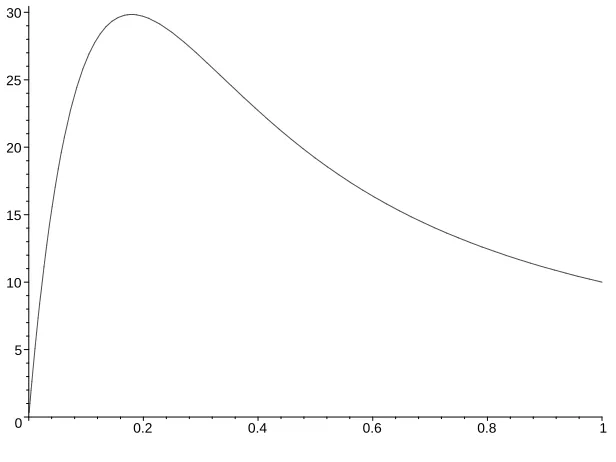
0 5 10 15 20 25 30
0.2 0.4 0.6 0.8 1
Figure 1: ϕ(p) =h(p)/p2 forD∼Po(10)andk=3.
Example 4.11. A standard case is whenD∼Po(λ)andk≥3. (This includes, as said above, the case
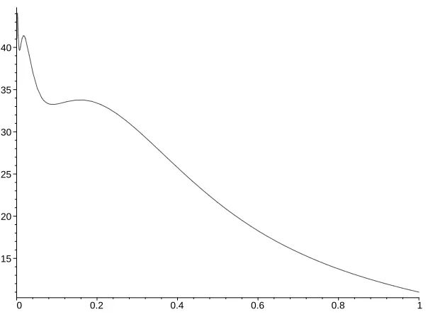
15 20 25 30 35 40
0 0.2 0.4 0.6 0.8 1
Figure 2: ϕ(p) =h(p)/p2 fork=3 and p10i =99·10−2i, i=1, 2, . . . , (pj =0 for all other j). Cf. Example 4.15.
59]. Hence, if ck := minµ>0µ/P(Po(µ) ≥ k−1) and λ > ck, then πc = inf0<p≤1 λp2/h(p)
= ck/λ. Moreover, it is easily shown thath(p)/p2 is unimodal, see[10, Lemma 7.2] and Figure 1. Consequently, there is as discussed above a single first-order phase transition atπ=ck/λ[17].
Example 4.12. Let k = 3 and consider graphs with only two vertex degrees, 3 and m, say, with
m≥4. Then, cf. (4.4),
h(p) =3p3P(Dp=3|D=3) +pmE(Dp−Dp1[Dp≤2]|D=m)
=3p3p3+pm mp−mp(1−p)m−1−m(m−1)p2(1−p)m−2.
Now, letp3:=1−a/mandpm:=a/m, witha>0 fixed andm≥a, and letm→ ∞. Then, writing
h=hm,hm(p)→3p3+apforp∈(0, 1]and thus
ϕm(p):=
hm(p)
p2 →ϕ∞(p):=3p+
a p.
Since ϕ∞′ (1) = 3−a, we see that if we choose a = 1, say, then ϕ∞′ (1) > 0. Furthermore, then ϕ∞(1/4) = 34 +4> ϕ∞(1) =4. Since alsoϕ′m(1) =3p3−mpm=3p3−a→ϕ∞′ (1), it follows that ifmis large enough, thenϕ′m(1)>0 butϕm(1/4)> ϕm(1). We fix such anmand note thatϕ=ϕm is continuous on[0,1]withϕ(0) =0, because the sum in (4.2) is finite with each termO(p3). Let ˜p0 be the global maximum point of ϕ in [0,1]. (If not unique, take the largest value.) Then,
by the properties just shown, ˜p0 6=0 and ˜p0 =6 1, so ˜p0 ∈(0, 1); moreover, 1 is a local maximum
point but not a global maximum point. Hence,πc=λ/ϕ(˜p0)is a first-order phase transition where the 3-core suddenly becomes non-empty and containing a positive fractionh1(˜p0)of all (remaining)
if ˜p1 := sup{p < 1 :ϕ(p) > ϕ(1)}, then ˜p1 < 1. Hence, as π ր 1, bp(π) ր ˜p1 and h(bp(π))ր h1(˜p1)<1. Consequently, the size of the 3-core jumps again atπ=1.
For an explicit example, numerical calculations (using Maple) show that we can take a = 1 and
m=12, ora=1.9 andm=6.
Example 4.13. Letk=3 and letDbe a mixture of Poisson distributions:
P(D= j) =pj=X
i
qiP(Po(λi) =j), j≥0, (4.18)
for some finite or infinite sequences(qi) and(λi)withqi ≥0, P
iqi =1 and λi ≥ 0. In the case
D∼Po(λ)we have, cf. Example 4.11,Dp∼Po(λp)and thus
h(p) =EDp−P(Dp=1)−2P(Dp=2) =λp−λpe−λp−(λp)2e−λp = (λp)2f(λp),
where f(x):= 1−(1+x)e−x/x. Consequently, by linearity, forDgiven by (4.18),
h(p) =X
i
qi(λip)2f(λip), (4.19)
and thus
ϕ(p) =X
i
qiλ2i f(λip). (4.20)
As a specific example, takeλi=2i andqi =λ−i 2=2−2i,i≥1, and addq0=1−
P
i≥1qiandλ0=0
to makePqi=1. Then
ϕ(p) =
∞ X
i=1
f(2ip). (4.21)
Note that f(x) =O(x) and f(x) =O(x−1) for 0< x < ∞. Hence, the sum in (4.21) converges uniformly on every compact interval[δ, 1]; moreover, if we define
ψ(x):=
∞ X
i=−∞
f(2ix), (4.22)