El e c t ro n ic
Jo ur
n a l o
f P
r o
b a b il i t y
Vol. 14 (2009), Paper no. 39, pages 1117–1161. Journal URL
http://www.math.washington.edu/~ejpecp/
The Virgin Island Model
Martin Hutzenthaler
∗†Johann Wolfgang Goethe-University Frankfurt
Rober-Mayer-Straße 10
60325 Frankfurt, Germany
Email: [email protected]
Abstract
A continuous mass population model with local competition is constructed where every emi-grant colonizes an unpopulated island. The population founded by an emiemi-grant is modeled as excursion from zero of an one-dimensional diffusion. With this excursion measure, we construct a process which we call Virgin Island Model. A necessary and sufficient condition for extinction of the total population is obtained for finite initial total mass.
Key words: branching populations, local competition, extinction, survival, excursion measure, Virgin Island Model, Crump-Mode-Jagers process, general branching process.
AMS 2000 Subject Classification:Primary 60K35, 92D25.
Submitted to EJP on October 9, 2008, final version accepted April 22, 2009.
∗Research supported by the DFG in the Dutch German Bilateral Research Group "Mathematics of Random Spatial
Models from Physics and Biology" (FOR 498)
1
Introduction
This paper is motivated by an open question on a system of interacting locally regulated diffusions. In[8], a sufficient condition for local extinction is established for such a system. In general, however, there is no criterion available for global extinction, that is, convergence of the total mass process to zero when started in finite total mass.
The method of proof for the local extinction result in[8]is a comparison with a mean field model
(Mt)t≥0which solves
d Mt =κ(EMt−Mt)d t+h(Mt)d t+ p
2g(Mt)d Bt (1)
where (Bt)t≥0 is a standard Brownian motion and where h,g:[0,∞)→R are suitable functions
satisfyingh(0) =0= g(0). This mean field model arises as the limit asN → ∞ (see Theorem 1.4 in[19]for the caseh≡0) of the following system of interacting locally regulated diffusions on N
islands with uniform migration
d XtN(i) =κ1
N
N−1
X
j=0
XtN(j)−XtN(i)
d t
+h XtN(i)
d t+Æ2g XtN(i)
d Bt(i) i=0, . . . ,N−1.
(2)
For this convergence, X0N(0), . . . ,X0N(N −1) may be assumed to be independent and identically distributed with the law of X0N(0) being independent of N. The intuition behind the comparison with the mean field model is that if there is competition (modeled through the functionshand g
in (2)) among individuals and resources are everywhere the same, then the best strategy for survival of the population is to spread out in space as quickly as possible.
The results of[8]cover translation invariant initial measures and local extinction. For generalhand
g, not much is known about extinction of the total mass process. Let the solution(XtN)t≥0 of (2) be started inX0N(i) = x1i=0, x≥0. We prove in a forthcoming paper under suitable conditions on the
parameters that the total mass|XtN| :=PNi=1XtN(i)converges as N → ∞. In addition, we show in that paper that the limiting process dominates the total mass process of the corresponding system of interacting locally regulated diffusions started in finite total mass. Consequently, a global extinction result for the limiting process would imply a global extinction result for systems of locally regulated diffusions.
In this paper we introduce and study a model which we callVirgin Island Modeland which is the limiting process of (XNt )t≥0 as N → ∞. Note that in the process(XtN)t≥0 an emigrant moves to a given island with probability N1. This leads to the characteristic property of the Virgin Island Model namely every emigrant moves to an unpopulated island. Our main result is a necessary and sufficient condition (see (28) below) for global extinction for the Virgin Island Model. Moreover, this condition is fairly explicit in terms of the parameters of the model.
Now we define the model. On the 0-th island evolves a diffusionY = (Yt)t≥0 with state spaceR≥0
given by the strong solution of the stochastic differential equation
d Yt =−a(Yt)d t+h(Yt)d t+p2g(Yt)d Bt, Y0= y≥0, (3)
where(Bt)t≥0is a standard Brownian motion. This diffusion models the total mass of a population
and the offspring variance are regulated by the total population. Later, we will specify conditions ona,hand gso thatY is well-defined. For now, we restrict our attention to the prototype example of a Feller branching diffusion with logistic growth in which a(y) = κy, h(y) = γy(K− y) and
g(y) =βy withκ,γ,K,β >0. Note that zero is a trap for Y, that is,Yt=0 implies Yt+s =0 for all
s≥0.
Mass emigrates from the 0-th island at rate a(Yt)d t and colonizes unpopulated islands. A new population should evolve as the process(Yt)t≥0. Thus, we need the law of excursions ofY from the trap zero. For this, define the set of excursions from zero by
U :=
χ∈C (−∞,∞),[0,∞)
:T0∈(0,∞],χt=0 ∀t∈(−∞, 0]∪[T0,∞) (4)
whereTy=Ty(χ):=inf{t>0:χt= y}is the first hitting time of y∈[0,∞). The setU is furnished with locally uniform convergence. Throughout the paper,C(S1,S2)andD(S1,S2)denote the set of continuous functions and the set of càdlàg functions, respectively, between two intervalsS1,S2⊂R.
Furthermore, define
D:=
χ∈D (−∞,∞),[0,∞)
:χt =0 ∀t<0 . (5)
Theexcursion measure QY is aσ-finite measure onU. It has been constructed by Pitman and Yor[16]
as follows: UnderQY, the trajectories come from zero according to an entrance law and then move according to the law ofY. Further characterizations ofQY are given in[16], too. For a discussion on the excursion theory of one-dimensional diffusions, see[18]. We will give a definition ofQY
later.
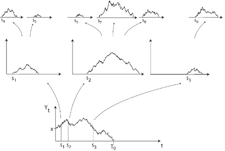
Next we construct all islands which are colonized from the 0-th island and call these islands the first generation. Then we construct the second generation which is the collection of all islands which have been colonized from islands of the first generation, and so on. Figure 1 illustrates the resulting tree of excursions. For the generation-wise construction, we use a method to index islands which keeps track of which island has been colonized from which island. An island is identified with a triple which indicates its mother island, the time of its colonization and the population size on the island as a function of time. Forχ∈D, let
I0χ :=
;, 0,χ (6)
be a possible 0-th island. For eachn≥1 andχ∈D, define
Inχ :=
ιn−1,s,ψ
:ιn−1∈ I
χ
n−1,(s,ψ)∈[0,∞)×D (7)
which we will refer to as the set of all possible islands of then-th generation with fixed 0-th island
(;, 0,χ). This notation should be read as follows. The island ιn = (ιn−1,s,ψ) ∈ I
χ
n has been colonized from islandιn−1 ∈ I
χ
n−1 at time sand carries total mass ψ(t−s) at time t ≥ 0. Notice
that there is no mass on an island before the time of its colonization. The island space is defined by
I :={;} ∪[
χ∈D
Iχ where Iχ := [
n≥0
Inχ. (8)
Denote byσι:=sthe colonization time of islandιifι= (ι
′
,s,ψ)for someι′∈ I. Furthermore, let
{Πι:ι∈ I \ {;}}be a set of Poisson point processes on[0,∞)×Dwith intensity measure
E
Π(ι,s,χ)(d t⊗dψ)
=a χ(t−s)
Figure 1: Subtree of the Virgin Island Model. Only offspring islands with a certain excursion height are drawn. Note that infinitely many islands are colonized e.g. between timess1ands2.
For later use, letΠχ := Π(;,0,χ). We assume that the family{Πι:ι ∈ Iχ}is independent for every χ∈D.
The Virgin Island Model is defined recursively generation by generation. The 0-th generation only consists of the 0-th island
V(0):=
;, 0,Y . (10)
The(n+1)-st generation,n≥0, is the (random) set of all islands which have been colonized from islands of then-th generation
V(n+1):=
ιn,s,ψ
∈ I:ιn∈ V(n),Πιn {(s,ψ)}
>0 . (11)
The set of all islands is defined by
V := [
n≥0
V(n). (12)
The total mass process of the Virgin Island Model is defined by
Vt:= X
ι,s,ψ∈V
ψ(t−s), t≥0. (13)
Our main interest concerns the behaviour of the lawL Vt
The following observation is crucial for understanding the behavior of (Vt)t≥0 as t → ∞. There is an inherent branching structure in the Virgin Island Model. Consider as new “time coordinate” the number of island generations. One offspring island together with all its offspring islands is again a Virgin Island Model but with the path(Yt)t≥0 on the 0-th island replaced by an excursion path. Because of this branching structure, the Virgin Island Model is a multi-type Crump-Mode-Jagers branching process (see [10] under “general branching process”) if we consider islands as individuals and[0,∞)×Das type space. We recall that a single-type Crump-Mode-Jagers process is a particle process where every particleigives birth to particles at the time points of a point process ξi until its death at timeλi, and(λi,ξi)i are independent and identically distributed. The literature on Crump-Mode-Jagers processes assumes that the number of offspring per individual is finite in every finite time interval. In the Virgin Island Model, however, every island has infinitely many offspring islands in a finite time interval becauseQY is an infinite measure.
The most interesting question about the Virgin Island Model is whether or not the process survives with positive probability as t→ ∞. Generally speaking, branching particle processes survive if and only if the expected number of offspring per particle is strictly greater than one, e.g. the Crump-Mode-Jagers process survives if and only ifEξi[0,λi]>1. For the Virgin Island Model, the offspring of an island(ι,s,χ)depends on the emigration intensitiesa χ(t−s)
d t. It is therefore not surpris-ing that the decisive parameter for survival is the expected “sum” over those emigration intensities
Z Z ∞
0
a χt
d t QY(dχ). (14)
We denote the expression in (14) as “expected total emigration intensity” of the Virgin Island Model. The observation that (14) is the decisive parameter plus an explicit formula for (14) leads to the following main result. In Theorem 2, we will prove that the Virgin Island Model survives with strictly positive probability if and only if
Z ∞
0
a(y)
g(y)exp
Z y
0
−a(u) +h(u)
g(u) du
d y>1. (15)
Note that the left-hand side of (15) is equal toR∞
0 a(y)m(d y)where m(d y) is the speed measure
of the one-dimensional diffusion (3). The method of proof for the extinction result is to study an integral equation (see Lemma 5.3) which the Laplace transform of the total mass V solves. Furthermore, we will show in Lemma 9.8 that the expression in (14) is equal to the left-hand side of (15).
Condition (15) already appeared in [8] as necessary and sufficient condition for existence of a nontrivial invariant measure for the mean field model, see Theorem 1 and Lemma 5.1 in[8]. Thus, the total mass process of the Virgin Island Model dies out if and only if the mean field model (1) dies out. The following duality indicates why the same condition appears in two situations which seem to be fairly different at first view. Ifa(x) =κx,h(x) =γx(K−x)and g(x) =βx withκ,γ,β >0, that is, in the case of Feller branching diffusions with logistic growth, then model (2) is dual to itself, see Theorem 3 in[8]. If(XtN)t≥0 indeed approximates the Virgin Island Model asN → ∞, then – for this choice of parameters – the total mass process(Vt)t≥0is dual to the mean field model. This duality would directly imply that – in the case of Feller branching diffusions with logistic growth – global extinction of the Virgin Island Model is equivalent to local extinction of the mean field model.
we give an expression in terms ofa,handg. In addition, in the critical case and in the supercritical case, we obtain the asymptotic behaviour of the expected area under the path ofV up to timet
Z t
0
ExVsds (16)
as t → ∞ for all x ≥ 0. More precisely, the order of (16) is O(t) in the critical case. For the supercritical case, letα >0 be the Malthusian parameter defined by
Z ∞
0
e−αu
Z
a χu
QY(dχ)du=1. (17)
It turns out that the expression in (16) grows exponentially with rateαas t→ ∞.
The result of Theorem 3 in the supercritical case suggests that the event that(Vt)t≥0 grows expo-nentially with rateαast→ ∞has positive probability. However, this is not always true. Theorem 7 proves thate−αtVt converges in distribution to a random variableW ≥0. Furthermore, this variable is not identically zero if and only if
Z Z∞
0
a χs
e−αsds
log+
Z∞
0
a χs
e−αsds
QY(dχ)<∞ (18)
where log+(x):=max{0, log(x)}. This(xlogx)-criterion is similar to the Kesten-Stigum Theorem (see[14]) for multidimensional Galton-Watson processes. Our proof follows Doney[4]who estab-lishes an(xlogx)-criterion for Crump-Mode-Jagers processes.
Our construction introduces as new “time coordinate” the number of island generations. Readers being interested in a construction of the Virgin Island Model in the original time coordinate – for example in a relation betweenVt and(Vs)s<t – are referred to Dawson and Li (2003)[3]. In that paper, a superprocess with dependent spatial motion and interactive immigration is constructed as the pathwise unique solution of a stochastic integral equation driven by a Poisson point pro-cess whose intensity measure has as one component the excursion measure of the Feller branching diffusion. In a special case (see equation (1.6) in [3]with x(s,a,t) = a, q(Ys,a) = κYs(R) and
m(d a) = 1[0,1](a)d a), this is just the Virgin Island Model with (3) replaced by a Feller branching
diffusion, i.e.a(y) =κy, h(y) =0, g(y) =βy. It would be interesting to know whether existence and uniqueness of such stochastic integral equations still hold if the excursion measure of the Feller branching diffusion is replaced byQY.
Models with competition have been studied by various authors. Mueller and Tribe (1994)[15]and Horridge and Tribe (2004) [7] investigate an one-dimensional SPDE analog of interacting Feller branching diffusions with logistic growth which can also be viewed as KPP equation with branching noise. Bolker and Pacala (1997)[2]propose a branching random walk in which the individual mor-tality rate is increased by a weighted sum of the entire population. Etheridge (2004)[6]studies two diffusion limits hereof. The “stepping stone version of the Bolker-Pacala model” is a system of inter-acting Feller branching diffusions with non-local logistic growth. The “superprocess version of the Bolker-Pacala model” is an analog of this in continuous space. Hutzenthaler and Wakolbinger[8], motivated by[6], investigated interacting diffusions with local competition which is an analog of the Virgin Island Model but with mass migrating onZ
2
Main results
The following assumption guarantees existence and uniqueness of a strong[0,∞)-valued solution of equation (3), see e.g. Theorem IV.3.1 in[9]. Assumption A2.1 additionally requires that a(·) is essentially linear.
Assumption A2.1. The three functions a:[0,∞)→[0,∞), h:[0,∞)→Rand g:[0,∞)→[0,∞)
are locally Lipschitz continuous in[0,∞)and satisfy a(0) =h(0) =g(0) =0. The function g is strictly positive on(0,∞). Furthermore, h andpg satisfy the linear growth condition
lim sup x→∞
0∨h(x) +pg(x)
x <∞ (19)
where x∨y denotes the maximum of x and y. In addition, c1·x≤a(x)≤c2·x holds for all x≥0and
for some constants c1,c2∈(0,∞).
The key ingredient in the construction of the Virgin Island Model is the law of excursions of(Yt)t≥0
from the boundary zero. Note that under Assumption A2.1, zero is an absorbing boundary for (3), i.e.Yt=0 impliesYt+s=0 for alls≥0. As zero is not a regular point, it is not possible to apply the well-established Itô excursion theory. Instead we follow Pitman and Yor[16]and obtain aσ-finite measure ¯QY – to be called excursion measure – on U (defined in (4)). For this, we additionally assume that (Yt)t≥0 hits zero in finite time with positive probability. The following assumption formulates a necessary and sufficient condition for this (see Lemma 15.6.2 in[13]). To formulate the assumption, we define
¯
s(z):=exp
−
Z z
1
−a(x) +h(x)
g(x) d x
, S¯(y):=
Z y
0
¯
s(z)dz, z,y >0. (20)
Note that ¯Sis a scale function, that is,
Py Tb(Y)<Tc(Y)
=
¯
S(y)−S¯(c)
¯
S(b)−S¯(c) (21)
holds for all 0≤c< y<b<∞, see Section 15.6 in[13].
Assumption A2.2. The functions a, g and h satisfy
Z x
0
¯
S(y) 1
g(y)¯s(y)d y<∞ (22)
for some x>0.
Note that if Assumption A2.2 is satisfied, then (22) holds for all x>0.
We carry out this construction in detail in Section 9. In addition Pitman and Yor[16]describe the excursion measure “in a preliminary way as”
lim y→0
1 ¯
S(y)L
y(Y) (23)
where the limit indicates weak convergence of finite measures on C [0,∞),[0,∞)
away from neighbourhoods of the zero-trajectory. However, they do not give a proof. Having ¯QY identified as the limit in (23) will enable us to transfer explicit formulas for L (Y) to explicit formulas for
¯
QY. We establish the existence of the limit in (23) in Theorem 1 below. For this, let the topology onC [0,∞),[0,∞)
be given by locally uniform convergence. Furthermore, recallY from (3), the definition ofU from (4) and the definition of ¯Sfrom (20).
Theorem 1. Assume A2.1 and A2.2. Then there exists aσ-finite measureQ¯Y on U such that
lim y→0
1 ¯
S(y)E
yF(Y) = Z
F(χ)Q¯Y(dχ) (24)
for all bounded continuous F:C [0,∞),[0,∞)
→ R for which there exists an ǫ > 0 such that
F(χ) =0wheneversupt≥0χt< ǫ.
For our proof of the global extinction result for the Virgin Island Model, we need the scaling function ¯
Sin (24) to behave essentially linearly in a neighbourhood of zero. More precisely, we assume ¯S′(0)
to exist in(0,∞). From definition (20) of ¯S it is clear that a sufficient condition for this is given by the following assumption.
Assumption A2.3. The integralRǫ1−a(gy()+y)h(y)d y has a limit in(−∞,∞)asǫ→0.
It follows from dominated convergence and from the local Lipschitz continuity of a and h that Assumption A2.3 holds ifR01 g(yy)d y is finite.
In addition, we assume that the expected total emigration intensity of the Virgin Island Model is finite. Lemma 9.6 shows that, under Assumptions A2.1 and A2.2, an equivalent condition for this is given in Assumption A2.4.
Assumption A2.4. The functions a, g and h satisfy
Z ∞
x
a(y)
g(y)¯s(y)d y<∞ (25)
for some and then for all x>0.
We mention that if Assumptions A2.1, A2.2 and A2.4 hold, then the process Y hits zero in finite time almost surely (see Lemma 9.5 and Lemma 9.6). Furthermore, we give a generic example for a, hand g namely a(y) = c1y, h(y) = c2yκ1−c3yκ2, g(y) = c4yκ3 with c1,c2,c3,c4 > 0.
The Assumptions A2.1, A2.2, A2.3 and A2.4 are all satisfied if κ2 > κ1 ≥ 1 and if κ3 ∈ [1, 2).
Assumption A2.2 is not met by a(y) =κy, κ >0, h(y) = y and g(y) = y2 because then ¯s(y) =
Next we formulate the main result of this paper. Theorem 2 proves a nontrivial transition from extinction to survival. For the formulation of this result, we define
s(z):=exp− Z z
0
−a(x) +h(x)
g(x) d x
, S(y):=
Z y
0
s(z)dz, z,y >0, (26)
which is well-defined under Assumption A2.3. Note that ¯S(y) =S(y)S¯′(0). Define the excursion measure
QY :=S¯′(0)Q¯Y (27)
and recall the total mass process(Vt)t≥0 from (13).
Theorem 2. Assume A2.1, A2.2, A2.3 and A2.4. Then the total mass process(Vt)t≥0 started in x>0
dies out (i.e., converges in probability to zero as t→ ∞) if and only if
Z ∞
0
a(y)
g(y)s(y)d y≤1. (28)
If (28)fails to hold, then Vt converges in distribution as t → ∞to a random variable V∞satisfying
Px(V∞=0) =1−Px(V∞=∞) =Exexp−q
Z ∞
0
a(Ys)ds (29)
for all x≥0and some q>0.
Remark 2.1. The constant q > 0 is the unique strictly positive fixed-point of a function defined in Lemma 7.1.
In the critical case, that is, equality in (28),Vt converges to zero in distribution ast→ ∞. However, it turns out that the expected area under the graph of V is infinite. In addition, we obtain in Theorem 3 the asymptotic behaviour of the expected area under the graph of V up to time t as
t→ ∞. For this, define
wa(x):=
Z ∞
0
S(x∧z) a(z)
g(z)s(z)dz, x ≥0, (30)
and similarly wid := wa with a(z) = z. If Assumptions A2.1, A2.2, A2.3 and A2.4 hold, then
wa(x) +wid(x) is finite for fixed x < ∞; see Lemma 9.6. Furthermore, under Assumptions A2.1, A2.2, A2.3 and A2.4,
w′a(0) =
Z ∞
0
a(z)
g(z)s(z)dz<∞ (31)
by the dominated convergence theorem.
Theorem 3. Assume A2.1, A2.2, A2.3 and A2.4. If the left-hand side of (28)is strictly smaller than
one, then the expected area under the path of V is equal to
Ex
Z ∞
0
Vsds=wid(x) +
w′id(0)wa(x)
for all x ≥ 0. Otherwise, the left-hand side of (32)is infinite. In the critical case, that is, equality in(28),
1
t
Z t
0
ExVsds→ w
′
id(0)wa(x) R∞
0
wa(y)
g(y)s(y)d y
∈[0,∞) as t→ ∞ (33)
where the right-hand side is interpreted as zero if the denominator is equal to infinity. In the supercritical case, i.e., if (28)fails to be true, letα >0be such that
Z ∞
0
e−αs
Z
a χs
QY(dχ)ds=1. (34)
Then the order of growth of the expected area under the path of(Vs)s≥0 up to time t as t→ ∞can be read off from
e−αt
Z t
0
ExVsds→ R∞
0 e
−αsR
χsQY(dχ)ds· R∞
0 e
−αsExa(Y s)ds
R∞
0
αse−αsR
a(χs)QY(dχ)
ds ∈
(0,∞) (35)
for all x≥0.
The following result is an analog of the Kesten-Stigum Theorem, see[14]. In the supercritical case,
e−αtVt converges to a random variableW as t → ∞. In addition, W is not identically zero if and only if the(xlogx)-condition (18) holds. We will prove a more general version hereof in Theorem 7 below. Unfortunately, we do not know of an explicit formula in terms of a, hand g for the left-hand side of (18). Aiming at a condition which is easy to verify, we assume instead of (18) that the second momentR(R∞
0 a(χs)ds)
2Q(dχ)is finite. In Assumption A2.5, we formulate a condition
which is slightly stronger than that, see Lemma 9.8 below.
Assumption A2.5. The functions a, g and h satisfy
Z ∞
x
a(y)y+wa(y)
g(y)¯s(y) d y<∞ (36)
for some and then for all x>0.
Theorem 4. Assume A2.1, A2.2, A2.3 and A2.5. Suppose that(28)fails to be true (supercritical case)
and letα >0be the unique solution of (34). Then
Vt eαt
w
−→W as t→ ∞ (37)
in the weak topology andP{W>0}=P{V∞>0}.
3
Outline
we obtain a criterion for survival and extinction in terms ofQY. More precisely, we prove that the process dies out if and only if the expression in (14) is smaller than or equal to one. In this step, we do not exploit thatQY is the excursion measure ofY. In fact, we will prove an analog of Theorem 2 in a more general setting whereQY is replaced by someσ-finite measureQand where the islands are counted with random characteristics. See Section 4 below for the definitions. The analog of Theorem 2 is stated in Theorem 5, see Section 4, and will be proven in Section 7. The key equation for its proof is contained in Lemma 5.1 which formulates the branching structure in the Virgin Island Model. In the second step, we calculate an expression for (14) in terms ofa,hand g. This will be done in Lemma 9.8. Theorem 2 is then a corollary of Theorem 5 and of Lemma 9.8, see Section 10. Similarly, a more general version of Theorem 3 is stated in Theorem 6, see Section 4 below. The proofs of Theorem 3 and of Theorem 6 are contained in Section 10 and Section 6, respectively. As mentioned in Section 1, a rescaled version of (Vt)t≥0 converges in the supercritical case. This
convergence is stated in a more general formulation in Theorem 7, see Section 4 below. The proofs of Theorem 4 and of Theorem 7 are contained in Section 10 and in Section 8, respectively.
4
Virgin Island Model counted with random characteristics
In the proof of the extinction result of Theorem 2, we exploit that one offspring island together with all its offspring islands is again a Virgin Island Model but with a typical excursion instead of
Y on the 0-th island. For the formulation of this branching property, we need a version of the Virgin Island Model where the population on the 0-th island is governed byQY. More generally, we replace the lawL (Y)of the first island by some measureν and we replace the excursion measure
QY by some measureQ. Given two σ-finite measuresν and Q on the Borel-σ-algebra of D, we define the Virgin Island Model with initial island measure ν and excursion measure Q as follows. Define the random sets of islandsV(n),ν,Q,n≥0, andVν,Q through the definitions (9), (10), (11) and (12) withL (Y) andQY replaced byν andQ, respectively. A simple example forν andQ is ν(dχ) =Q(dχ) =Eδt7→1t<L
(dχ)where L≥0 is a random variable andδψis the Dirac measure on
the pathψ. Then the Virgin Island Model coincides with a Crump-Mode-Jagers process in which a particle has offspring according to a ratea(1)Poisson process until its death at time L.
Furthermore, our results do not only hold for the total mass process (13) but more generally when the islands are counted with random characteristics. This concept is well-known for Crump-Mode-Jagers processes, see Section 6.9 in [10]. Assume that φι = φι(t)
t∈R
, ι ∈ I, are separable and nonnegative processes with the following properties. It vanishes on the negative half-axis, i.e. φι(t) =0 for t <0. Informally speaking our main assumption onφι is that it does not depend on
the history. Formally we assume that
φ ι,s,χ(t)
t∈R
d
=φ
;,0,χ(t−s)
t∈R
∀χ∈D,ι∈ I,s≥0. (38)
Furthermore, we assume that the family {φι,Πι:ι ∈ Iχ} is independent for each χ ∈ D and
(ω,t,χ)7→φ(;,0,χ)(t)(ω)is measurable. As a short notation, defineφχ(t):=φ(t,χ):=φ(;,0,χ)(t) forχ∈D. With this, we define
Vtφ,ν,Q:= X
ι∈Vν,Q
and say that Vtφ,ν,Q
t≥0 is a Virgin Island process counted with random characteristics φ. Instead
ofVtφ,δχ,Q, we write Vtφ,χ,Q for a path χ ∈D and note that(ω,t,χ) 7→Vtφ,χ,Q(ω) is measurable. A prominent example for φχ is the deterministic random variable φχ(t) ≡ χ(t). In this case, Vtν,Q := Vtφ,ν,Q is the total mass of all islands at time t. Notice that (Vt)t≥0 defined in (13) is a special case hereof, namelyVt = VL
(Y),QY
t . Another example forφχ isφ(t,χ) =χ(t)1t
≤t0. Then
Vtφ,χ,Q is the total mass at timet of all islands which have been colonized in the lastt0 time units.
Ifφ(t,χ) =R∞
t χsds, thenV
φ,χ,Q
t =
R∞ t V
χ,Q s ds.
As in Section 2, we need an assumption which guarantees finiteness ofVtφ,ν,Q.
Assumption A4.1. The function a:[0,∞)→[0,∞)is continuous and there exist c1,c2∈(0,∞)such that c1x≤a(x)≤c2x for all x ≥0. Furthermore,
sup t≤T
Z
a χt
+Eφ t,χ
ν(dχ) +sup t≤T
Z
a χt
+Eφ t,χ
Q(dχ)<∞ (40)
for every T <∞
The analog of Assumption A2.4 in the general setting is the following assumption.
Assumption A4.2. Both the expected emigration intensity of the0-th island and of subsequent islands
are finite:
Z Z ∞
0
a χu
du
ν(dχ) +
Z Z ∞
0
a χu
du
Q(dχ)<∞. (41)
In Section 2, we assumed that(Yt)t≥0hits zero in finite time with positive probability. See Assump-tion A2.2 for an equivalent condiAssump-tion. Together with A2.4, this assumpAssump-tion implied almost sure convergence of(Yt)t≥0 to zero as t → ∞. In the general setting, we need a similar but somewhat
weaker assumption. More precisely, we assume thatφ(t) converges to zero ”in distribution“ both with respect toν and with respect toQ.
Assumption A4.3. The random processes
φχ(t)
t≥0:χ∈D and the measures Q andν satisfy
Z
1−Ee−λφ(t,χ) ν+Q
(dχ)→0 as t→ ∞ (42)
for allλ≥0.
Having introduced the necessary assumptions, we now formulate the extinction and survival result of Theorem 2 in the general setting.
Theorem 5. Letν be a probability measure onDand let Q be a measure on D. Assume A4.1, A4.2
and A4.3. Then the Virgin Island process(Vtφ,ν,Q)t≥0counted with random characteristicsφwith0-th island distributionν and with excursion measure Q dies out (i.e., converges to zero in probability) if and only if
¯
a:=
Z Z ∞
0
a χu
In case of survival, the process converges weakly as t→ ∞to a probability measureL V∞φ,ν,Q
on the point∞where q>0is the unique strictly positive fixed-point of
z7→
Remark 4.1. The assumption onν to be a probability measure is convenient for the formulation in
terms of convergence in probability. For a formulation in the case of aσ-finite measureν, see the proof of the theorem in Section 7.
Next we state Theorem 3 in the general setting. For its formulation, define
fν(t):=
Z
Eφ(t,χ)ν(dχ), t≥0, (46)
and similarly fQ withν replaced byQ.
Theorem 6. Assume A4.1 and A4.2. If the left-hand side of (43)is strictly smaller than one and if both fν and fQ are integrable, then
which is finite and strictly positive. Otherwise, the left-hand side of (47)is infinite. If the left-hand side of (43)is equal to one and if both fν and fQare integrable,
where the right-hand side is interpreted as zero if the denominator is equal to infinity. In the supercritical case, i.e., if (43)fails to be true, letα >0be such that
Additionally assume that fQis continuous a.e. with respect to the Lebesgue measure,
∞ time t can be read off from
and from
lim t→∞e
−αt Z
E
Vtφ,χ,Q
ν(dχ) =
R∞
0 e
−αsfQ(s)ds
·R0∞e−αsRa χs
ν(dχ)ds
R∞
0 se−
αsR
a χs
Q(dχ)ds
. (52)
For the formulation of the analog of the Kesten-Stigum Theorem, denote by
¯
m:=
R∞
0 e
−αsfQ(s)ds
R∞
0 se−
αsR
a χs
Q(dχ)ds ∈
(0,∞) (53)
the right-hand side of (52) withν replaced byQ. Furthermore, define
Aα(χ):=
Z ∞
0
a χs
e−αsds (54)
for every pathχ∈D. For our proof of Theorem 7, we additionally assume the following properties ofQ.
Assumption A4.4. The measure Q satisfies
Z Z T
0
a(χs)ds
2
Q(dχ)<∞ (55)
for every T <∞and
sup t≥0
Z
Eφχ(t)
Z t
0
a χs
ds
Q(dχ)<∞, sup t≥0
Z
E φχ2(t)
Q(dχ)<∞. (56)
Theorem 7. Letν be a probability measure onD and let Q be a measure onD. Assume A4.1, A4.2,
A4.3 and A4.4. Suppose that¯a>1(supercritical case) and letα >0be the unique solution of (49). Then
Vtφ,ν,Q eαtm¯
w
−→W as t→ ∞ (57)
in the weak topology where W is a nonnegative random variable. The variable W is not identically zero if and only if
Z
Aα(χ)log+ Aα(χ)
Q(dχ)<∞ (58)
wherelog+(x):=max{0, log(x)}. If (58)holds, then
EW=
Z hZ ∞
0
e−αsa χs
ds
i
ν(dχ),P W =0
=
Z h
e−q
R∞
0 a(χs)ds i
ν(dχ) (59)
where q>0is the unique strictly positive fixed-point of (45).
Remark 4.2. Comparing(59)with(44), we see that P(W >0) =P(V∞φ,ν,Q >0). Consequently, the Virgin Island process Vtφ,ν,Q
t≥0 conditioned on not converging to zero grows exponentially fast with
5
Branching structure
We mentioned in the introduction that there is an inherent branching structure in the Virgin Island Model. One offspring island together with all its offspring islands is again a Virgin Island Model but with a typical excursion instead ofY on the 0-th island. In Lemma 5.1, we formalize this idea. As a corollary thereof, we obtain an integral equation for the modified Laplace transform of the Virgin Island Model in Lemma 5.3 which is the key equation for our proof of the extinction result of Theorem 2. Recall the notation of Section 1 and of Section 4.
Lemma 5.1. Letχ∈D. There exists an independent family
n
(s,ψ)Vφ,χ,Q t
t≥0:(s,ψ)∈[0,∞)×D
o
(60)
of random variables which is independent ofφχ and ofΠχ such that
Vtφ,χ,Q=φχ(t) +
X
(s,ψ)∈Πχ
(s,ψ)Vφ,χ,Q
t ∀t≥0 (61)
and such that
(s,ψ)Vφ,χ,Q t
t≥0
d
=Vtφ−,sψ,Q
t≥0 (62)
for all(s,ψ)∈[0,∞)×D.
Proof. WriteVχ :=Vχ,Q andV(n),χ:=V(n),χ,Q. Define
(s,ψ)
V(1),χ :=n (;, 0,χ),s,ψo
⊂ I1χ and
(s,ψ)
Vχ :=[
n≥1
(s,ψ)
V(n),χ (63)
for(s,ψ)∈[0,∞)×Dwhere
(s,ψ)
V(n+1),χ :=n ιn,r,ζ
∈ Inχ+1:ιn∈(s,ψ)V(n),χ,Πιn(r,ζ)>0 o
(64)
forn≥1. Comparing (63) and (64) with (11), we see that
V(0),χ =
(;, 0,χ) and V(n),χ = [
(s,ψ)∈Πχ
(s,ψ)
V(n),χ ∀n≥1. (65)
DefineVt(0),φ,χ,Q=φχ(t)fort≥0 and forn≥1
Vt(n),φ,χ,Q:= X
(s,ψ)∈Πχ
X
ι∈(s,ψ)V(n),χ
φι(t−σι) =:
X
(s,ψ)∈Πχ
(s,ψ)V(n),φ,χ,Q
t . (66)
Summing overn≥0 we obtain fort≥0
Vtφ,χ,Q=φχ(t) +
X
(s,ψ)∈Πχ
X
n≥1
(s,ψ)V(n),φ,χ,Q
t =:φχ(t) +
X
(s,ψ)∈Πχ
(s,ψ)Vφ,χ,Q
This is equality (61). Independence of the family (60) follows from independence of(Πι)ι∈Iχ and
from independence of(φι)ι∈Iχ. It remains to prove (62). Because of assumption (38) the random
characteristicsφι only depends on the last part ofι. Therefore
(s,ψ)V(n),φ,χ,Q
· =
X
ι∈(s,ψ)V(n),χ
φι · −σι
d
= X
˜ι∈V(n−1),ψ,Q
φ˜ι(· −(σ˜ι+s)) =V
(n−1),ψ,Q ·−s .
(68)
Summing overn≥1 results in (62) and finishes the proof.
In order to increase readability, we introduce the following suggestive symbolic abbreviation
I
h
f Vtφ,ν,Qi :=
Z
Ef Vtφ,χ,Q
ν(dχ) t ≥0,f ∈C [0,∞),[0,∞)
. (69)
One might want to read this as “expectation” with respect to a non-probability measure. However, (69) is not intended to define an operator.
The following lemma proves that the Virgin Island Model counted with random characteristics as defined in (39) is finite.
Lemma 5.2. Assume A4.1. Then, for every T<∞,
sup t≤T
I
h
Vtφ,ν,Q
i
<∞. (70)
Furthermore, if
sup t≤T
Z
E φ2χ(t)
+
Z T
0
a(χs)ds
2
Q(dχ)<∞, (71)
then there exists a constant cT <∞such that
sup t≤T
I
Vtφ,ν,Q
2
≤cT1+sup t≤T
Z
E φχ2(t)
(ν+Q)(dχ) +
Z Z T
0
a(χs)ds
2
ν(dχ)
(72)
for allν and the right-hand side of (72)is finite in the special caseν=Q.
Proof. We exploit the branching property formalized in Lemma 5.1 and apply Gronwall’s inequality.
Recall V(n),χ,Q from the proof of Lemma 5.1. The two equalities (66) and (68) imply
I
h
Vt(0),φ,ν,Q
i
=
Z
Eφχ(t)ν(dχ)≤sup
s≤T Z
fort≤T and forn≥1
Using Assumption A4.1 induction onn≥0 shows that all expressions in (73) and in (74) are finite in the caseν =Q. Summing (74) overn≤n0we obtain
fort≤T. In the special caseν=QGronwall’s inequality implies
n0
for some ˜cT <∞. In addition the two equalities (66) and (68) together with independence imply
In the special caseν=Qinduction onn≥0 together with (71) shows that all involved expressions are finite. A similar estimate as in (79) leads to
Z
In the special caseν=QGronwall’s inequality together with (77) leads to
Z
which is finite by Assumption A4.1 and assumption (71). Inserting (80) into (79) and lettingn0→
∞finishes the proof.
In the following lemma, we establish an integral equation for the modified Laplace transform of the Virgin Island Model. Recall the definition ofVtφ,ν,Q from (39).
Lemma 5.3. Assume A4.1. The modified Laplace transformI
1−e−λVtφ,ν,Qof the Virgin Island Model
counted with random characteristicsφsatisfies
I
6
Proof of Theorem 6
Recall the definition of(Vtφ,ν,Q)t≥0from (39), fν from (46) and the notationIfrom (69). We begin with the supercritical case and letα >0 be the Malthusian parameter which is the unique solution of (49). Define
mν(t):=IhVtφ,ν,Qi µν(ds):=
Z
a χs
ν(dχ)ds (82)
fort≥0. In this notation, equation (74) withν replaced byQreads as
e−αtmQ(t) =e−αtfQ(t) +
Z t
0
e−α(t−s)mQ(t−s)e−αsµQ(ds). (83)
This is a renewal equation for e−αtmQ(t). By definition ofα, e−αsµQ(ds)is a probability measure. From Lemma 5.2 we know thatmQis bounded on finite intervals. By assumption, fQis continuous Lebesgue-a.e. and satisfies (50). Hence, we may apply standard renewal theory (e.g. Theorem 5.2.6 of[10]) and obtain
lim t→∞e
−αtmQ(t) = R∞
0 e
−αsfQ(s)ds
R∞
0 se−
αsµQ(ds) <∞. (84)
Multiply equation (74) by e−αt, recall e−αtfν(t)→0 as t → ∞and apply the dominated conver-gence theorem together with A4.2 to obtain
lim t→∞e
−αtmν(t) =
Z ∞
0
e−αs lim t→∞e
−α(t−s)mQ(t
−s)µν(ds). (85)
Insert (84) to obtain equation (52). An immediate consequence of the existence of the limit on the left-hand side of (85) is equation (51)
e−αt
Z t
0
mν(s)ds=
Z ∞
0
e−αs·e−α(t−s)mν(t−s)ds−−→t→∞ 1
α·tlim→∞e
−αtmν(t) (86)
where we used the dominated convergence theorem.
Next we consider the subcritical and the critical case. Define
¯
xν(t):=
Z t
0
IhVsφ,ν,Q
i
ds, t≥0. (87)
In this notation, equation (74) integrated over[0,t]reads as
¯
xν(t) =
Z t
0
fν(s)ds+
Z t
0
¯
xQ(t−u)µν(du), t≥0. (88)
In the subcritical case, fQ and fν are integrable. Theorem 5.2.9 in [10] applied to (88) withν replaced byQimplies
lim t→∞¯x
Q(t) = R∞
0 f
Q(s)ds
Lettingt→ ∞in (88), dominated convergence andµν [0,∞)
<∞imply
lim t→∞x¯
ν(t) =
Z ∞
0
fν(s)ds+
Z ∞
0
lim t→∞¯x
Q(t
−u)µν(du). (90)
Inserting (89) results in (47). In the critical case, similar arguments lead to
lim t→∞
1
tx¯ ν(t)
= lim t→∞
1
t
Z t
0
fν(s)ds+
Z ∞
0
lim t→∞
t−u t tlim→∞
1
t−ux¯
Q(t
−u)µν(du)
=
R∞
0 f
Q(s)ds
R∞
0 uµ
Q(du)µ
ν [0, ∞)
.
(91)
The last equality follows from (88) withν replaced by Q and Corollary 5.2.14 of[10]with c :=
R∞
0 f
Q(s)ds,n:=0 andθ :=R∞
0 uµ
Q(du). Note that the assumptionθ <∞of this corollary is not
necessary for this conclusion.
7
Extinction and survival in the Virgin Island Model. Proof of
Theo-rem 5
Recall the definition of (Vtφ,ν,Q)t≥0 from (39) and the notationIfrom (69). As we pointed out in Section 2, the expected total emigration intensity of the Virgin Island Model plays an important role. The following lemma provides us with some properties of the modified Laplace transform of the total emigration intensity. These properties are crucial for our proof of Theorem 5.
Lemma 7.1. Assume A4.2. Then the function
k(z):=
Z
1−exp−z
Z ∞
0
a χs
dsQ(dχ), z≥0, (92)
is concave with at most two fixed-points. Zero is the only fixed-point if and only if
k′(0) =
Z Z ∞
0
a χs
ds Q(dχ)≤1. (93)
Denote by q the maximal fixed-point. Then we have for all z≥0:
z≤k(z) =⇒ z≤q (94)
z≥k(z)∧z>0 =⇒ z≥q. (95)
Proof. IfR0∞a χs
ds =0 forQ-a.a.χ, then k≡0 and zero is the only fixed-point. For the rest of
the proof, we assume w.l.o.g. thatR R∞
0 a(χs)ds
The functionkhas finite values because of 1−e−c≤c,c≥0, and Assumption A4.2. Concavity ofk
is inherited from the concavity of x 7→1−e−x c,c≥0. Using dominated convergence together with Assumption A4.2, we see that
k(z)
z =
Z 1
−exp −zR0∞a(χs)ds
z Q(dχ)
z→∞
−−→0. (96)
In addition, dominated convergence together with Assumption A4.2 implies
k′(z) =
Z hZ ∞
0
a χs
dsexp−z
Z ∞
0
a χs
dsiQ(dχ) z≥0. (97)
Hence,kis strictly concave. Thus,khas a fixed-point which is not zero if and only ifk′(0)>1. The implications (94) and (95) follow from the strict concavity ofk.
The method of proof (cf. Section 6.5 in [10]) of the extinction result for a Crump-Mode-Jagers process (Jt)t≥0 is to study an equation for (Ee−λJt)
t≥0,λ≥0. The Laplace transform (Ee−λJt)λ≥0
converges monotonically toP(Jt =0)asλ→ ∞,t ≥0. Furthermore,P(Jt=0) =P(∃s≤t:Js=0)
converges monotonically to the extinction probabilityP(∃s≥0:Js=0)ast→ ∞. Taking monotone limits in the equation for(Ee−λJt)
t≥0,λ≥0results in an equation for the extinction probability. In our
situation, there is an equation for the modified Laplace transform(Lt(λ))t>0,λ>0 as defined in (98) below. However, the monotone limit ofLt(λ)asλ→ ∞might be infinite. Thus, it is not clear how to transfer the above method of proof. The following proof of Theorem 2 directly establishes the convergence of the modified Laplace transform.
Proof of Theorem 5. Recallqfrom Lemma 7.1. In the first step, we will prove
Lt:=Lt(λ):=I
1−e−λVtφ,Q,Q→q (as t→ ∞) (98)
for allλ >0. Set Lt(0):=0. It follows from Lemma 5.2 that(Lt)t≤T is bounded for every finiteT. Lemma 5.3 withν replaced byQprovides us with the fundamental equation
Lt= Z
E
h
1−exp
−λφχ(t)−
Z ∞
0
a χs
Lt−sds i
Q(dχ) ∀t≥0. (99)
Based on (99), the idea for the proof of (98) is as follows. The termλφχ(t)vanishes as t→ ∞. If Lt converges to some limit, then the limit has to be a fixed-point of the function
k(z) =
Z h
1−exp−z
Z ∞
0
a χs
dsiQ(dχ). (100)
We will need finiteness of L∞:=lim supt→∞Lt. Looking for a contradiction, we assume L∞=∞.
The last summand converges to zero by Assumption A4.3 and is therefore bounded by some constant
c. Inequality (101) leads to the contradiction
1≤ lim
calculation as in (101) results in
lim
The last summand is equal to zero by Assumption A4.3. The first summand on the right-hand side of (103) is dominated by
which is finite by boundedness of(Lt)t≥0 and by Assumption A4.2. Applying dominated conver-gence, we conclude thatL∞is bounded by
Using dominated convergence, the assumptionm=0 results in the contradiction
with dominated convergence yields
m= lim
Finally, we finish the proof of Theorem 5. Applying Lemma 5.3, we see that
The first summand on the right-hand side of (109) converges to zero ast→ ∞by Assumption A4.3. By the first step (98), Lt → q as t → ∞. Hence, by the dominated convergence theorem and Assumption A4.2, the left-hand side of (109) converges to zero as t → ∞. As ν is a probability measure by assumption, we conclude
lim
This implies Theorem 5 as the Laplace transform is convergence determining, see e.g. Lemma 2.1 in[5].
8
The supercritical Virgin Island Model. Proof of Theorem 7
nevertheless include here for the reason of completeness. Lemma 8.9 and Lemma 8.10 below con-tain the essential part of the proof of Theorem 7. For these two lemmas, we will need auxiliary lemmas which we now provide.
We assume throughout this section that a solutionα∈Rof equation (34) exists. Note that this is
implied by A4.2 andQ R0∞a(χs)ds>0
>0. Recall the definition ofµQ from (82).
8.1
Preliminaries
Forλ≥0, define
Hα(ψ)(λ):=
Z h
1−exp− Z ∞
0
a χs
ψ(λe−αs)dsiQ(dχ) (111)
forψ∈D.
Lemma 8.1. The operator Hα is contracting in the sense that
Hα(ψ1)(λ)−Hα(ψ2)(λ) ≤
Z ∞
0
ψ1(λe−αs)−ψ2(λe−αs)
µQ(ds) (112)
for allψ1,ψ2∈D.
Proof. The lemma follows immediately from|e−x −e−y| ≤ |x−y|and from the definition (82) of µQ.
Lemma 8.2. The operator Hα is nondecreasing in the sense that
Hα(ψ1)(λ)≤Hα(ψ2)(λ) (113)
for allλ≥0ifψ1(λ)≤ψ2(λ)for allλ≥0.
Proof. The lemma follows from 1−e−c x being increasing inx for everyc>0.
For every measurable functionψ:R×[0,∞)→[0,∞), define
¯
Hα(ψ)(t,λ):=
Z
f
Z ∞
0
a χs
ψ(t−s,λe−αs)ds
Q(dχ). (114)
forλ≥0 and t ∈Rwhere f(x):= x−1+e
−x
≥0, x ≥0. If ˜ψ:[0,∞)→[0,∞)is a function of one variable, then we set ¯Hα(ψ˜)(λ):=H¯α(ψ)(1,λ)whereψ(t,λ):=ψ˜(λ)forλ≥0,t∈R.
Lemma 8.3. The operatorH¯α is nondecreasing in the sense that
¯
Hα(ψ1)(t,λ)≤H¯α(ψ2)(t,λ) (115)
for allλ≥0and t∈Rifψ1(t,λ)≤ψ2(t,λ)for allλ≥0, t∈R.
Lemma 8.4. Assume A4.2. Let id:λ7→λbe the identity map. The function
η(λ):=1− 1
λHα(id)(λ) = 1
λH¯α(id)(λ), λ >0, (116)
is nonnegative and nondecreasing. Furthermore,η(0+) =0.
Proof. Recall the definition ofAα(χ)from (54). By equation (114), we haveλη(λ) =
R
f(λAα)dQ.
Thus,ηis nonnegative. Furthermore,η(0+) =0 follows from the dominated convergence theorem and Assumption A4.2. Letx,y>0. Then
η(x+y)−η(x) =
Z
xAαf (x+y)Aα
−(x+y)Aαf xAα
x(x+y)Aα dQ≥0. (117)
The inequality follows from ˜x f(x˜+˜y)−(˜x+˜y)f(˜x)≥0 for all ˜x, ˜y≥0.
The following lemma, due to Athreya[1], translates the(xlogx)-condition (58) into an integrability condition onη. For completeness, we include its proof.
Lemma 8.5. Assume A4.2. Letηbe the function defined in(116). Then
Z
0+ 1
λη(λ)dλ <∞and ∞ X
n=1
η(c rn)<∞ (118)
for some and then all c>0, r<1if and only if the(xlogx)-condition(58)holds.
Proof. By monotonicity ofη(see Lemma 8.4), the two quantities in (118) are finite or infinite at the
same time. Fixc>0. Using Fubini’s theorem and the substitutionv:=λAα, we obtain
Z c
0
1
λη(λ)dλ=
Z Z c
0
hλAα−1+e−λAα
(λAα)2
i
Aα
2
dλ
dQ
=
Z
Aα
Z cAα
0
v−1+e−v
v2 d v
dQ.
(119)
It is a basic fact thatRT
0 1
v2(v−1+e− v)d v
∼logT asT → ∞.
8.2
The limiting equation
In the following two lemmas, we consider uniqueness and existence of a functionΨwhich satisfies:
(a) Ψ(λ1)−Ψ(λ2)
≤ |λ1−λ2|forλ1,λ2≥0, Ψ(0) =0 (b) Ψ(λ) =Hα(Ψ)(λ)
(c) Ψ(λ)
λ →1 asλ→0
(d) 0≤Ψ(λ1)≤Ψ(λ2)≤λ2 ∀0≤λ1≤λ2and lim
λ→∞Ψ(λ) =q
(120)