www.elsevier.nl / locate / econbase
The effects of the unemployment insurance payroll tax
on wages, employment, claims and denials
a b ,*
Patricia M. Anderson , Bruce D. Meyer a
Department of Economics, Dartmouth College, Hanover, NH, USA b
Department of Economics and, Institute for Policy Research, Northwestern University, 2003 Sheridan Road, Evanston, IL 60208-2600, USA
Received 1 August 1998; received in revised form 1 December 1998; accepted 1 January 1999
Abstract
Following a 13-year period when all employers in Washington paid the same unemploy-ment insurance (UI) tax rate, Washington was forced to adopt an experience-rated tax system in 1985. We use this ‘‘natural experiment’’ to explore both tax incidence and the effects of experience rating. We find that industry average tax rates are largely passed on to workers through lower earnings. However, our estimates imply that a firm can shift much less of the difference between its tax rate and the industry average rate. Our results also indicate that experience rating reduces turnover and UI claims, and increases claim denials.
2000 Elsevier Science S.A. All rights reserved.
Keywords: Unemployment insurance; Payroll taxes; Incidence; Experience rating; Claim administra-tion; Labor demand
JEL classification: H22; J65
1. Introduction
The recent experience of Washington State provides a natural setting to examine the effects of the unemployment insurance payroll tax. During the 13-year period from 1972 through 1984, all employers in Washington paid the same
unemploy-*Corresponding author. Tel.:11-847-491-8226; fax:11-847-491-7001.
E-mail address: [email protected] (B.D. Meyer).
ment insurance (UI) tax rate, but a by-product of Federal legislation then forced Washington to adopt an experience-rated system. In March of 1984, the state passed legislation that made a firm’s tax rate a function of its past use of UI, resulting in a wide range of tax rates beginning in 1985. Thus, a comparison of wages, employment, claims and denials before and after the change has the potential to provide good evidence both on tax incidence and on the effects of experience rating.
More generally, this ‘‘natural experiment’’ provides evidence on several broader economic issues. First, many programs and employer mandates besides UI impose payroll taxes or tax-like costs on firms. The effects of these taxes or costs on wages and employment are central to the calculation of efficiency and equity
1
consequences of policies. Second, many such situations involve taxes or costs that vary across firms within the same labor market, as do UI taxes. The implications of a tax vary greatly depending on whether the tax is uniform across all firms in a
2
market or differs within markets. Differences in taxes across firms competing in the same labor and product markets cannot be shifted to wages or prices, and thus can be expected to have substantial employment effects. Third, experience rating imposes costs on firms that use layoffs to adjust their employment level. Thus, the evidence in this paper also has implications for the study of labor demand with
3
adjustment costs.
The effects of UI taxes are also an important policy issue in their own right. For several reasons, UI taxes are a potential candidate for reform. For example, with an extremely low tax base, the tax is very regressive. Also, the tax leads to
4
substantial interfirm and interindustry subsidies. Perhaps most importantly, the imperfections in current experience rating systems may lead to more layoffs and higher unemployment than would occur under more complete experience rating. In fact, several authors attribute a substantial share of temporary layoff
unemploy-5
ment to incomplete experience rating. Similarly, experience rating provides an incentive for firms to be involved in the administration of benefit claims. While information on this effect of experience rating is scant, it is often argued that experience rating makes employers more likely to examine whether UI claims are
6
justified. Finally, it is important to realize that the issues of incidence and layoff
1
For example, see Gruber and Krueger (1991); Hamermesh (1993); Aaron and Bosworth (1994). 2
See Anderson and Meyer (1997). 3
See Nickell (1986) and Hamermesh (1993) for surveys, and Anderson (1993) for a study of the role of UI.
4
See Becker (1972); Munts and Asher (1981), and for recent evidence Anderson and Meyer (1993). 5
By incomplete experience rating we mean that employers are not charged the full UI costs of a layoff. See Saffer (1982), Topel (1983, 1986), Card and Levine (1994), and Anderson and Meyer (1994).
6
incentives are linked, because experience-rated increases in taxes do not provide an incentive to reduce layoffs if they can be passed on easily to workers or consumers.
The experience of Washington State should also provide direct evidence on the effects other countries might expect from a decision to move to an experience-rated UI system. Although the increased administrative requirements of experience rating are sometimes mentioned as a drawback to such a shift, all fifty states have overcome these difficulties. Indeed, this feat has been accomplished despite the relatively high levels of firm and worker turnover in the U.S. While such a system might seem alien to many countries, the U.S. UI system is similar to certain existing institutions in other countries. In particular, many countries experience rate other types of insurance, such as that for workplace accidents. Other countries also impose severance payments for worker layoffs, leading to adjustment costs similar to those incurred as a result of experience rating.
This ‘‘natural experiment’’ analysis makes several advances over previous studies. First, past work on the incidence of taxes has rarely had available longitudinal earnings that permit one to account for unobserved differences between workers. Second, past work has not had clearly identified tax changes that applied to certain readily identified groups and not to others. It has also been harder in the past to argue that any tax differences were exogenous to the outcomes of interest. Third, previous work on experience rating has often used proxies for firm incentives and differences across states that were potentially correlated with firm preferences for layoffs. The forced reintroduction of ex-perience rating in Washington State provides a way to overcome these problems. Using this large policy change to estimate the incidence of the UI tax generally confirms the basic implications from past work. In our preferred specifications, we find that the market-level tax is largely passed on to the worker in the form of lower earnings. However, our estimates further imply that the firm can shift much less of the firm-level tax. Our estimates of changes in UI claim rates and in seasonal employment variation agree with the prediction that experience rating reduces layoffs. Also, our results for claim denial rates suggest that under experience rating, firms contest more claims. In the next section, we discuss the changes to the Washington State UI payroll tax system that have taken place over the past 15 years. Section 3 presents a brief outline of the theoretical models motivating the empirical work, while Section 4 presents the tax incidence estimates. Section 5 presents the experience rating estimates, and Section 6 then concludes.
2. The Washington state UI payroll tax system
state legislation would have brought back experience rating if the state UI fund balance reached a high level, this event was not expected to occur in the
7
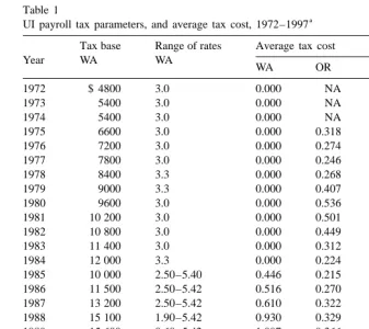
foreseeable future. This system meant that, in practice, there was no experience rating for 13 years. The Tax Equity and Fiscal Responsibility Act of 1982 (TEFRA) required all states to have a maximum rate of at least 5.4 percent by 1985. A uniform tax rate of 5.4 percent, however, would have heavily overtaxed most firms in Washington and generated a huge tax surplus. Thus, this federal requirement led the state legislature in March 1984 to pass a law that reinstated experience rating beginning in 1985. The state adopted a benefit ratio system of experience rating with a series of tax schedules (more detail is provided in Appendix A). The schedule in force in a given year depended on the state UI trust fund balance. Combined with Washington’s fairly high tax base ($12 000 in 1984), this policy shift led to a dramatic change in both marginal UI costs and the distribution of taxes paid across firms. A quick summary of the main characteris-tics of the Washington State UI payroll tax over this period can be found in Table 1. The table reports the tax base and the range of tax rates for the years 1972–1997.
At the time of the reintroduction of experience rating, there were some other
8
less important changes in Washington’s UI law. The tax base was temporarily lowered, as can be seen in Table 1. The automatic annual increase in the maximum weekly benefit was suspended for one year. A provision was then passed that first came into effect in 1989 that raised the maximum benefit from 55 percent of average wages to 60 percent. There was also a very minor one-year change in the continuing eligibility requirements for those with a marginal labor force attach-ment. None of these changes should be important for our analyses, except for the tax base change, which we account for below.
As can be seen in the table, the changes in taxes were substantial. From 1984 to 1985 some firms saw an increase in their tax rate from 3.0 to 5.4 percent, while others saw a decrease from 3.0 to 2.5 percent. Incorporating the decrease in the tax base, firm tax payments may have risen or fallen between 36 and 37% in nominal
9
dollars. The range of tax rates widened further by 1989, when some firms saw an increase in their tax to 5.42 percent, while others saw a decrease to 0.60 percent. We examine the incidence of the UI tax, however, using the initial 1984–1985 large change in payroll taxes.
The changes in the Washington tax schedule also affected the level of experience rating in the state, allowing us to examine the effect of experience
7
This summary of expectations can be found in Washington State Employment Security (1984). In fact, an employment security official in charge of legislative issues indicated to one of the authors that he thought that the old tax system would still be in place if not for the federal legislation.
8
Two Washington State Employment Security Department law descriptions, Washington State Employment Security (undated (a), undated (b)), provide a good summary.
9
Table 1
a UI payroll tax parameters, and average tax cost, 1972–1997
Tax base Range of rates Average tax cost
Year WA WA
WA OR ID
1972 $ 4800 3.0 0.000 NA 0.469
1973 5400 3.0 0.000 NA 0.454
1974 5400 3.0 0.000 NA 0.447
1975 6600 3.0 0.000 0.318 0.450
1976 7200 3.0 0.000 0.274 0.447
1977 7800 3.0 0.000 0.246 0.460
1978 8400 3.3 0.000 0.268 0.493
1979 9000 3.3 0.000 0.407 0.515
1980 9600 3.0 0.000 0.536 0.535
1981 10 200 3.0 0.000 0.501 0.540
1982 10 800 3.0 0.000 0.449 0.547
1983 11 400 3.0 0.000 0.312 0.581
1984 12 000 3.3 0.000 0.224 0.566
1985 10 000 2.50–5.40 0.446 0.215 0.545
1986 11 500 2.50–5.42 0.516 0.270 0.533
1987 13 200 2.50–5.42 0.610 0.322 0.552
1988 15 100 1.90–5.42 0.930 0.329 0.551
1989 15 600 0.60–5.42 1.097 0.366 0.524
1990 16 200 0.50–5.42 1.117 0.491 0.517
1991 16 800 0.50–5.42 1.352 0.605 0.499
1992 17 600 0.50–5.42 1.361 0.560 0.495
1993 18 500 0.50–5.42 1.585 0.465 0.485
1994 19 900 0.36–5.40 1.295 0.343 0.468
1995 19 900 0.36–5.40 0.878 0.410 0.458
1996 20 300 0.36–5.40 0.833 0.480 0.570
1997 21 300 0.36–5.40 0.889 0.531 0.452
a
Sources: ET Handbook No. 394, Commerce Clearing House Unemployment Insurance Reports, Significant Provisions of State Unemployment Insurance Laws, Highlights of State Unemployment Compensation Laws, unpublished tabulations from State UI administrations, and authors’ calculations.
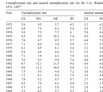
Table 2
Unemployment rate and insured unemployment rate for the U.S., Washington, Oregon, and Idaho, a
1972–1997
Year Unemployment rate Insured unemployment rate
US WA OR ID US WA OR ID
1972 5.6 9.5 5.7 6.2 3.2 6.5 4.0 3.6
1973 4.9 7.9 6.2 5.6 2.9 5.7 3.7 3.2
1974 5.6 7.2 7.5 6 5.0 6.4 4.6 3.8
1975 8.5 9.3 10.2 7.4 4.9 8.4 7.2 5.3
1976 7.6 8.7 9.5 5.7 4.4 7.0 5.4 4.4
1977 7.1 8.8 7.4 5.9 3.7 5.7 4.6 3.9
1978 6.1 6.9 6.1 5.6 3.2 3.4 3.4 3.0
1979 5.8 6.8 6.8 5.7 3.2 2.9 3.4 3.5
1980 7.1 7.9 8.3 7.9 3.6 4.6 5.4 5.2
1981 7.6 9.5 9.9 7.6 4.0 4.9 5.9 5.1
1982 9.7 12.1 11.5 9.8 4.8 6.8 7.4 7.3
1983 9.6 11.2 10.8 9.8 3.2 5.6 5.5 5.6
1984 7.5 9.5 9.4 7.2 3.0 4.3 4.2 4.2
1985 7.2 8.1 8.8 7.9 2.9 4.4 4.6 4.5
1986 7.0 8.2 8.5 8.7 2.7 4.1 4.9 4.8
1987 6.2 7.6 6.2 8.0 2.2 3.7 3.5 4.2
1988 5.5 6.2 5.8 5.8 2.0 3.6 3.1 3.6
1989 5.3 6.2 5.7 5.1 2.3 3.6 3.4 3.9
1990 5.6 4.9 5.6 5.9 2.8 4.0 4.2 3.2
1991 6.8 6.4 6.1 6.2 3.1 4.0 4.2 3.8
1992 7.5 7.6 7.6 6.5 2.6 4.0 4.2 3.7
1993 6.9 7.6 7.3 6.2 2.6 3.9 3.8 3.3
1994 6.1 6.4 5.4 5.6 2.6 4.3 3.6 3.1
1995 5.6 6.4 4.8 5.4 2.5 4.0 3.3 3.2
1996 5.4 6.5 5.9 5.2 2.3 3.7 3.4 3.1
1997 4.9 4.8 5.8 5.3 NA NA NA NA
a
Sources: BLS web site, ET Handbook No. 394, and the Green Book.
Table 2 reports unemployment rates in the U.S., Washington State, and the neighboring states of Idaho and Oregon as background information. One can see that between 1984 and 1985 there were only small changes in the unemployment rate and in the insured unemployment rate in the jurisdictions listed in the table. One should note that the unemployment rate in Washington may have been slightly lower after 1984 due to the reintroduction of experience rating. One can also see that it is necessary to look back to the early 1970’s to find unemployment rates similar to those in 1996 and 1997.
3. Theory
due to the fact that firms are now experience rated. Depending on the incidence of the tax, changes in the after-tax cost of labor should lead to changes in wages, employment or both. Additionally, the move to experience rating, with its resultant change in the marginal cost of laying off a worker, should impact both the firm’s employment decision and the firm’s involvement in the administration of benefits. In the first case, changes in the marginal layoff incentives should alter the cyclicality and seasonality of employment and thus the prevalence of UI claims. In the second case, the implementation of experience rating should provide firms with an increased incentive to review claims and contest those that are not truly the result of a layoff.
3.1. Incidence
The incidence of a tax change is complicated if the change in the tax varies across firms. In previous work (Anderson and Meyer, 1997) we present a theoretical model which incorporates variation in firm taxes both within and across competitive labor markets. This model highlights the importance of distinguishing between the effects of a change in the market-level tax rate (measured as the industry average) and a change in a firm’s tax rate, holding the market-level tax rate constant. We also allow for the fact that the value of potential UI benefits affects a worker’s employment decision and note that transitory changes in taxes may be discounted by firms due to experience rating. We then show that an increase in the market-level tax rate reduces wages and employment, with the magnitude of these effects depending on the demand for labor, the supply of labor, the worker valuation of the benefits and the firm discounting of the tax.
The exogenous nature of the tax changes in Washington provides a clear advantage over the past work and also makes possible several simplifications to our general model. First, since the tax change did not directly alter the compensation for unemployment provided by UI, we do not have to account for the individual valuation of the benefits provided by UI or for how that valuation affects workers’ supply curves. Second, since the change was permanent, we do not need to account for firms’ discounting of the taxes they pay. The implication, then, is
≠Wf ] 50,
≠tf
and
d ≠Wf hm ]≠t 5]]]s d ,
h 2h
m m m
where W is a wage,t a tax rate,h an elasticity, f refers to the firm, m to the
21. Thus, the experience of Washington State should provide a natural setting to cleanly examine the incidence of the UI payroll tax.
3.2. Experience rating
The basis for expecting a move to experience rating to impact firm decisions comes from the fact that future tax payments are now directly linked to the amount of UI benefits that are received by former employees. As a result, incentives for the firm, both in terms of optimal employment decisions and involvement in benefit administration, have been altered. Turning first, then, to the effects of experience rating on firm employment decisions, theoretical models have generally followed one of two approaches (see Anderson and Meyer (1994) for a discussion). One approach treats UI as an adjustment cost, while the other treats UI as part of a compensation package. The adjustment cost approach notes that if a firm is responsible for paying part of the cost of the UI benefits generated by a layoff, the firm’s cost of adjusting the employment level is higher. Simple models of dynamic demand can be used to show that if the firm would otherwise vary employment over time, this cost would cause the firm to smooth employment somewhat more than it would otherwise. Thus, peak employment will be lower,
10
and trough employment will be higher. Such a reduction in the variation in
employment will therefore imply fewer layoffs and UI claims.
The alternative approach to investigating the effect of experience rating on firm employment decisions treats UI as part of an overall compensation package. Firms are assumed to offer workers a combination of paid work and UI supported leisure, providing a level of utility equal to the market offer. Profits are thus maximized subject to this utility constraint. In a perfectly experience-rated system, each firm would be responsible for the payments to its laid-off workers. Since with imperfect experience rating firms pay only a fraction of each dollar received by these workers, the system provides a subsidy for this component of compensation relative to wages. Thus, temporary layoffs should be higher the larger this subsidy,
11
i.e. the lower the degree of experience rating.
These two approaches can also be combined, as in Anderson and Meyer (1994), by extending a simple adjustment cost model, in which product demand de-terministically fluctuates between good and bad states, to include endogenous wages. Wages would then be determined by the constraint that firms must provide a wage / UI package that supplies a level of utility equal to that in alternative employment. In this case, tighter experience rating is associated with fewer layoffs and UI claims and a reduction in their variation over time. With either approach, though, one can generally predict that the effect of experience rating on the firm’s
10
See Anderson (1993) for evidence of this effect on seasonal employment at retail trade firms and Card and Levine (1994) for evidence over the business cycle.
11
employment decision will lead to lower levels of layoffs and UI claims, decreased variability of employment and claims, and may change employment levels in either direction.
Turning now to the effect of experience rating on firm involvement in the administration of benefits, our last prediction is that experience rating will increase the probability that workers’ UI claims will be contested by employers and will increase the likelihood that claims are denied. Workers who quit their jobs or are fired for cause are not eligible for unemployment insurance. If the reason for a separation is not clear, the worker may claim that he was laid off, while the firm might believe that the worker quit or was fired. Firms may also contest the continuation of payments to claimants who have turned down suitable jobs. Without experience rating, employers do not have an incentive to contest such claims, since a former employee’s claim does not increase future tax payments for the firm. Under experience rating, UI claims charged to a firm increase that firm’s future taxes giving firms an incentive to contest claims. Thus, we expect that a change from no experience rating to experience rating should lead to a higher fraction of claims being contested, and thus denied. Perhaps less clear is whether such an increase in denials is clearly desirable. Becker (1972) provides some evidence that employer involvement in claims is beneficial, though this issue is often contested. In particular, it is argued that experience rating may lead employers to contest reasonable claims. Additionally, this increased employer involvement will lead to increases in the administrative resources devoted to
12
resolving disputes over claims. Overall, then, it is not clear that the benefits of
removing ineligible claimants from the rolls will outweigh the costs from errors and increased disputes. While we cannot examine the cost-benefit issue, we are able to examine whether experience rating increases claim denial rates as is predicted.
4. Empirical analysis of the incidence of the UI tax
In order to analyze the incidence of the UI tax, we use administrative data from the Washington State UI system. These data consist of quarterly earnings records for a ten percent random sample of covered individuals. In addition to the earnings received by the employee, the records contain a firm identifier. Based on this identifier, information on firm tax rates in 1985 has been appended to the individual data. A significant advantage of using panel data is that by differencing the data we can remove unmeasured characteristics of a firm’s working conditions and benefits package, as well as any unmeasured differences across individuals in
12
ability or tastes. This differencing thus removes factors which many previous authors have argued severely bias empirical estimates of wage determinants.
A drawback to the data is that despite their administrative source, they appear to
13
have significant errors. An examination of the consistency of the earnings and
hours numbers over time strongly suggests that there are recording errors. While hours worked in the quarter do appear on the earnings records, we have determined that their reliability is too low to be used in the analysis. As well as recording errors, another problem is that it is not clear precisely how this field is completed for workers who are not paid on an hourly basis. Since earnings in the quarter accord closely with payments made to workers, no matter the method used to compute pay, we feel this is a more reliable data field. Though we would prefer to use hourly earnings, we are forced to use quarterly earnings. Ideally, we would like to carry out an analysis at the firm level also, but the likely more reliable quarterly firm payroll information was unavailable for the period surrounding the
14
tax change.
In order to look at a change in taxes that is not a function of firm actions during the period of observation, we examine changes between the third or fourth quarters of 1984 (1984:Q3,Q4) and those from 1985 (1985:Q3,Q4). The 1985 tax rate was only determined by firm actions prior to the first period, specifically layoffs resulting in UI receipt between 1980:Q3 and 1984:Q2. While employers during 1984:Q3,Q4 had recently learned that a tax change was imminent, the details were only available at the end of the year. If there were fast adjustments in anticipation of the tax change, however, the result would likely be a bias towards zero in the tax effects. There are additional advantages to using just this change. First, looking at longer differences would greatly reduce the sample due to turnover, since we only use individuals remaining at the same firm across the different years. Second, looking at later one-year differences would mean relying on changes in tax rates due to behavior changes that occurred during the post-experience rating period. As a result, the changes in taxes would be less likely to be exogenous.
Prior to differencing the data, we remove all observations that are clearly identifiable as quarters in which a job match began or ended. Thus, if a quarter is the first appearance of a unique match of a firm and individual identifier, that observation is excluded. Similarly, if a quarter is the last appearance of the unique match, that observation is excluded. Additionally, quarters in which we can identify a temporary layoff by the presence of UI benefit receipt are also excluded. Unfortunately, temporary layoffs during which UI benefits are not received cannot be clearly identified. Thus, in addition to data errors, we also have some
13
The fact that individual-level data is not used by the UI system unless the worker applies for benefits implies that much of the data likely never undergo any serious quality checks.
14
unobserved temporary layoffs in the data. Below, we describe our approach to limiting the impact of such observations.
As was seen in Table 1, the firm does not pay its assigned tax rate on the entire payroll, but instead the tax base is only the first $12 000 per employee in 1984 and the first $10 000 in 1985. In addition, there is a small federal tax of 0.8% on a $7000 base. Since on average the taxable wage base is much lower than earnings, we must use an appropriate earnings measure to calculate the effective firm tax rate as a proportion of the wage bill. We use two such earnings measures, the actual quarterly earnings for the individual and average earnings in the market.
To define a market, we must rely on standard industrial classifications (SIC’s). While labor markets are probably best delineated by occupation or skill level, we rely on the correlation between industry and occupation and skill in defining markets. We experiment with several SIC classifications, starting by grouping similar 3-digit SIC’s into about 150 different industries. Alternatively, we estimate models using 2-digit SIC and 4-digit SIC classifications. In each case, we obtain market-level tax rates by calculating the average of the firm tax over all individual observations in the quarter within the grouped 3-digit industry. However, if there are less than 5 firms in the industry, all of the observations from that market are
15
dropped.
16
We use the change in the natural log of individual earnings between 1985 and
1984 as the dependent variable in our regressions, and thus estimate specifications of the general form: taxes for market m and firm f, respectively, and all other subscripts are defined analogously. Note that Ty, q,k5state ratey,k3[min(state base ,Wy y, q,i)]1federal ratey3[min(federal base ,Wy y, q,i)], where k is equal to f or m. The additional
covariates zy, q are a dummy for third quarter and dummies for a broader industry
17
grouping. In variations of this model, the market and firm tax measures are
15
This restriction is effective in both dropping the less accurate market tax rates and less competitive markets. This restriction also implies different sample sizes depending on the market definition.
16
Because of the concerns about data reporting errors and unidentified temporary separations discussed above, 6,664 individuals with changes outside of the range of20.5 to 0.5 are dropped for most of the analysis. An additional 102 individuals are dropped because their market no longer contains 5 firms after imposing the above restriction. Alternate methods of dealing with outliers are discussed below.
17
entered separately. As indicated above, alternative models, that substitute industry
average W for Wy, q,i on the right hand side of the equation, are also estimated.
This formulation of the effective tax rate builds in a mechanical endogeneity of the tax change variables from two sources. The first source is the presence of earnings in the denominator of each term. The second source of endogeneity is the fact that the tax bill increases with the earnings. To solve this endogeneity problem we use instrumental variables to estimate our models. We estimate models with two different sets of instruments. First, we instrument the change in tax variables with variables of the same form, but with
Wy, q,i1Wy21, q,i
]
]]]]]
Wq,i5
2
substituted for Wy, q,i and Wy21, q,i wherever they appear in the calculation of the
18
change in tax variables. These instruments are only a function of statutory
changes in the tax rates and tax base, and changes in the average wage level. Thus, it will be valid as long as the tax changes are exogenous and the wage change is unrelated to the wage level. In fact, this assumption is not strictly true, as a regression of the change in log earnings on the average individual earnings level yields a statistically significant coefficient. However, the magnitude of this relation is very small, being zero to the sixth decimal place. As an alternative, though, we also try instrumenting the change in tax variables with variables using only the change in the statutory tax rate. These instruments are clearly valid, but likely
19
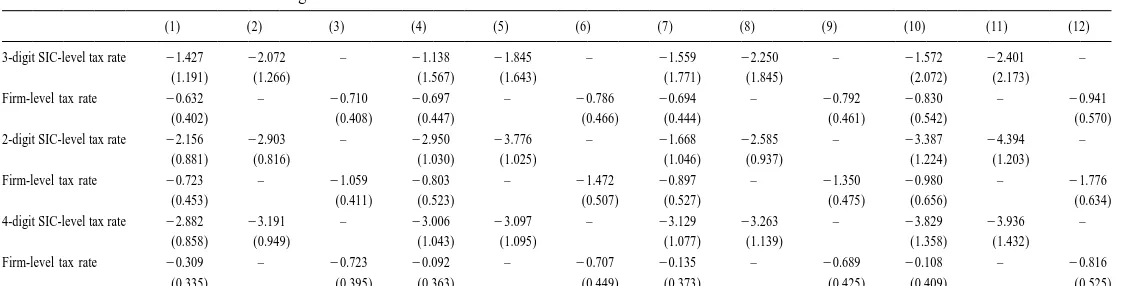
weaker, since they do not incorporate the level of or change in the tax base. Table 3 reports the results of estimating the above models, with the top panel showing the estimates using the individual earnings based tax rates and the bottom
20
panel those using the industry earnings based tax rates. Within each panel,
models are estimated using each of the three different market definitions and each of the two different instrument sets discussed above. In all cases, the standard
21
errors have been adjusted to account for the correlation within industry group. Although the estimates are relatively imprecise, some basic patterns do emerge. First, as expected, in all cases earnings fall with higher taxes. Second, no matter which earnings base is used in the tax variables or which variables are used as instruments, when entered jointly (i.e. models (1), (4), (7) and (10)) the point
18
When the tax change variable is defined based on average market earnings, the instrument is defined analogously.
19
In all cases the first-stage regressions are significant. For example, looking at the firm tax calculated with individual earnings, using the average wage-based instrument results in a first-stage coefficient (standard error) of 1.006 (0.002), while using the statutory change instrument gives us 0.566 (0.002). Results for other models are similar.
20
These same models were also estimated excluding firms with over 5000 workers in order to determine if one or two firms were exercising undue influence. In general, results were very similar to those reported here.
21
.
Anderson
,
B
.D
.
Meyer
/
Journal
of
Public
Economics
78
(2000
)
81
–
106
93
Table 3
a The effect of UI taxes on individual earnings
(1) (2) (3) (4) (5) (6) (7) (8) (9) (10) (11) (12)
3-digit SIC-level tax rate 21.427 22.072 – 21.138 21.845 – 21.559 22.250 – 21.572 22.401 – (1.191) (1.266) (1.567) (1.643) (1.771) (1.845) (2.072) (2.173)
Firm-level tax rate 20.632 – 20.710 20.697 – 20.786 20.694 – 20.792 20.830 – 20.941 (0.402) (0.408) (0.447) (0.466) (0.444) (0.461) (0.542) (0.570) 2-digit SIC-level tax rate 22.156 22.903 – 22.950 23.776 – 21.668 22.585 – 23.387 24.394 –
(0.881) (0.816) (1.030) (1.025) (1.046) (0.937) (1.224) (1.203)
Firm-level tax rate 20.723 – 21.059 20.803 – 21.472 20.897 – 21.350 20.980 – 21.776 (0.453) (0.411) (0.523) (0.507) (0.527) (0.475) (0.656) (0.634) 4-digit SIC-level tax rate 22.882 23.191 – 23.006 23.097 – 23.129 23.263 – 23.829 23.936 –
(0.858) (0.949) (1.043) (1.095) (1.077) (1.139) (1.358) (1.432)
Firm-level tax rate 20.309 – 20.723 20.092 – 20.707 20.135 – 20.689 20.108 – 20.816 (0.335) (0.395) (0.363) (0.449) (0.373) (0.425) (0.409) (0.525)
a
estimate of the effect of the market-level tax is greater than that of the firm-level tax. This result would be expected if competitive firms can mainly pass through shared costs. Additionally, in these models the point estimate on the firm-level tax is smaller the more narrow the market definition. Assuming that the increased homogeneity of a more narrow industry group is likely to correspond to groupings of firms that are more competitive in the labor market, this result is also as expected. While theoretically the firm-level tax should have a zero coefficient, there are several reasons why we might expect a non-zero coefficient. First, our imprecision in defining markets likely means that it partly captures the market-level tax. Second, since we must use earnings in place of wages, negative employment or hours effects could lead to an estimated negative effect on earnings.
While the basic patterns of the coefficients are consistent with the theory, the magnitude of the point estimates on the industry-level tax, whether entered jointly or alone, is larger than expected. However, it is mainly only in the 2-digit case, where the additional industry controls are likely less precise, that one cannot reject that the negative coefficient is less than 1 in absolute value. Recall that a
coefficient of21 would represent complete shifting of the market-level tax burden
to workers. Although the general findings are robust to the alternative instruments and earnings bases, it does appear that the estimates are relatively sensitive to the treatment of outliers.
Using the full sample, rather than dropping observations with a more than fifty percent change in earnings, leads to very different results from those reported. For example, focusing on model (1), the coefficient (standard error) on the 3-digit
SIC-level tax rate is 20.693 (1.847), while that on the firm-level tax rate is
21.172 (0.771). Similar differences can be seen for the other industry groups. For
the 2-digit SIC group, the industry and firm results are 22.501 (1.260) and
21.208 (0.796), respectively, while for the 4-digit SIC group the estimates are
24.114 (1.462) and 20.338 (0.661). Similar differences can be found for the
other models. It is clear that the point estimates are heavily influenced by what are likely data errors and undetected temporary separations.
We explore an alternative approach to dealing with the issue through the use of median regression. To carry out this experiment, we use the instruments from
22
Table 3 as the independent variables. Since it is plausible that the firm would
respond to tax measures based on the average of a worker’s earnings rather than on the actual worker’s earnings, the instrument is a reasonable explanatory variable. The differences between the original variables and instruments is extremely small, in any case. Thus, median regression can be justified on this basis. Additionally, this exploration can be thought of as a median regression version of indirect least squares. Given that the coefficients in the first stage for the
22
IV estimates are almost exactly one, indirect least squares is essentially the same as 2SLS, making the coefficients comparable.
Looking again at model (1), when estimated at the 3-digit level the firm-level
estimate, at 20.513, remains fairly similar to that in Table 3, but much less
23
negative than the 2SLS results for the same sample. The industry-level point
estimate of20.948 is between that in Table 3 and that obtained using 2SLS on the
full sample. The median regression results for the other industry groups are all much less negative than the 2SLS estimates using the same sample, and somewhat less negative than those in Table 3. The industry and firm coefficients for the
2-digit SIC group are 21.934 and 20.515, and for the 4-digit SIC group are
22.586 and 20.113. Results for the other models are similar. Overall, then, it
appears that median regression on the full sample and our approach using a restricted sample lead to similar conclusions. Our approach has the advantage, though, of simplifying the use of instruments and the adjustment of standard errors.
In addition to the possibility of outliers affecting the estimates, another consideration is that the broader industry group controls may not be sufficient to pick up differences in earnings trends, causing the market tax variable to pick up some of this trend in specifications (1)–(3) and (7)–(9). Recall that because of the low tax base, changes in taxes will be lower for the more highly paid. If at the same time wage growth is faster for the more highly paid, as may be the case
24
given increasing returns to skill, then we are likely to obtain estimates of the
market-level tax effect on earnings which are negatively biased. However, given that we are only looking at changes in earnings over a one year period, this impact of increasing inequality is unlikely to be extremely large, and this problem does not apply to specifications (4)–(6) and (10)–(12).
Overall, then, while large standard errors preclude us from drawing strong conclusions, it does appear that the firm is able to pass on a substantial part of the portion of the UI payroll tax that is shared by all firms in a market, but is somewhat less able to shift the firm-specific portion. Earlier work on the incidence of payroll taxes has been fairly inconclusive, though more recent work on mandated benefits has generally found that the costs can be passed on to
25
employees. However, since the tax change in Washington was driven by Federal
legislation and did not directly alter the compensation for unemployment provided by UI, our results are more applicable to payroll tax incidence, rather than to the
23
We do not report standard errors here because the standard calculation method will not account for the correlation within industry group, and our main focus is on the effect of outliers on the point estimates.
24
See, for example, Levy and Murnane (1992). 25
costs of financing a benefit. Additionally, the experience of Washington State provides a much cleaner source of changes in tax rates than does most past work.
5. Empirical analysis of the effects of UI experience rating
As was seen earlier, the implementation of experience rating is expected to impact several labor market variables, including UI claims and denials, and employment variability. Thus, we have collected data on several outcomes of interest for the period 1972 to 1997 from all 50 states and the District of
26
Columbia. The use of this panel allows us to fully exploit the change in the UI
system of Washington State by first performing a difference-in-differences analysis
27
on several variables. From the Department of Labor, Employment and Training
Administration, we obtained monthly data on initial claims and weeks claimed, and quarterly data on separation issue denials and nonseparation issue denials. We also obtained monthly information on employment from the Bureau of Labor
28
Statistics and annual population figures from the Census Bureau.
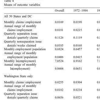
Our outcome variables are then created as follows. We first construct claim rates for each state by dividing monthly claims by monthly employment. Similarly, separation issue denial rates are constructed as the ratio of denials to claims, while nonseparation issue denial rates are constructed as the ratio of denials to weeks claimed. In both cases, the number of claims or number of weeks claimed is first aggregated to the quarterly level. Employment to population ratios are constructed by dividing monthly employment by the annual population figures for individuals age 18–64. Additional outcome variables include the log of monthly employment, along with the annual ranges of the monthly claim rate, the monthly employment to population ratio, and the log of monthly employment. Table 4 presents the means of the outcome variables, both overall and split between the period with no experience rating (1972–1984) and the period with experience rating (1985– 1997), for all 51 states combined, and for Washington only.
While simple difference-in-differences could be calculated from this table, they will not quite reflect the correct experiment, since Washington is included in the
29
top panel. Rather than making this simple comparison in means, however, we
will generally want to control for additional variables. In addition, we need to
26
For ease of exposition, we will hereafter refer to this panel as being made up of 51 states. 27
It is this desire for a control group, which allows us to difference out business cycle effects that leads us to choose to carry out this analysis on state-level data rather than attempting an analysis using the administrative data used above.
28
The URL addresses are http: / / stats.bls.gov / datahome.htm and http: / / www.census.gov / popula-tion / estimates / statepop.html for the employment and populapopula-tion figures respectively.
29
Table 4
Means of outcome variables
Overall 1972–1984 1985–1997 All 50 States and DC
Monthly claims / employment 0.0169 0.0198 0.0140 Annual range of monthly
claims / employment 0.0181 0.0215 0.0147 Quarterly separation issue
denials / quarterly claims 0.1126 0.1119 0.1132 Quarterly nonseparation issue
denials / weeks claimed 0.0185 0.0168 0.0202 Monthly employment / population 0.6824 0.6457 0.7222 Annual range of monthly
employment / population 0.0406 0.0415 0.0398 Monthly ln(employment) 7.0524 6.9162 7.1887 Annual range of monthly
ln(employment) 0.0604 0.0651 0.0558
Washington State only
Monthly claims / employment 0.0255 0.0304 0.0205 Annual range of monthly
claims / employment 0.0182 0.0234 0.0130 Quarterly separation issue
denials / quarterly claims 0.0656 0.0521 0.0794 Quarterly nonseparation issue
denials / weeks claimed 0.0168 0.0164 0.0171 Monthly employment / population 0.6375 0.5981 0.6801 Annual range of monthly
employment / population 0.0399 0.0393 0.0405 Monthly ln(employment) 7.4519 7.2466 7.6572 Annual range of monthly
ln(employment) 0.0632 0.0663 0.0602
Marginal tax cost 0.4964 0 0.9929
account for the likely dependence between observations from a given state and time period. The significance of results is commonly overstated in the natural experiment literature (and elsewhere) by not accounting for this type of
30
correlation. Thus, we obtain our difference-in-difference estimates from the
following two-step procedure. First, we run a regression of the form:
Yst5asDs1bs(D ds y.84)1gZ ,st (2)
where Y is one of the outcome variables described above for a given state andst
time period, D is a vector consisting of 51 dummy variables (one for each state),s
30
dy.84 is a dummy variable indicating the experience rated period (i.e. the years
1985–1997), and Z is a vector of control variables. The 51st b’s now represent the
corrected difference in the outcome variable for each state. We then run a weighted
31
least squares regression ofb on a dummy for Washington State. This coefficient
is the corrected difference-in-differences estimate of the impact of experience rating.
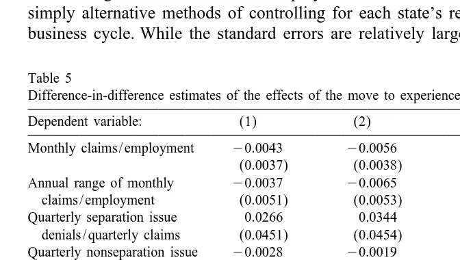
Table 5 presents the results for each of our outcome variables. Model (1) includes no control variables, and hence is identical to what would be obtained from a simple comparison of the difference in means for Washington minus the difference in means calculated over all states other than Washington. Model (2) includes the interaction of state dummies with the log of the monthly U.S. unemployment rate, while model (3) includes the interaction of state dummies
32
with the log of the annual state unemployment rate. Thus, models (2) and (3) are
simply alternative methods of controlling for each state’s response to the overall business cycle. While the standard errors are relatively large, the point estimates
Table 5
a Difference-in-difference estimates of the effects of the move to experience rating
Dependent variable: (1) (2) (3)
Monthly claims / employment 20.0043 20.0056 20.0031
(0.0037) (0.0038) (0.0029)
Annual range of monthly 20.0037 20.0065 20.0072 claims / employment (0.0051) (0.0053) (0.0046) Quarterly separation issue 0.0266 0.0344 0.0291
denials / quarterly claims (0.0451) (0.0454) (0.0438) Quarterly nonseparation issue 20.0028 20.0019 20.0015
denials / weeks claimed (0.0090) (0.0094) (0.0099) Monthly employment / population 0.0056 0.0066 20.0054
(0.0422) (0.0429) (0.0537)
Annual range of monthly 0.0030 0.0012 20.0042 employment / population (0.0072) (0.0071) (0.0071)
Monthly Ln(employment) 0.1408 0.1485 0.1501
(0.1200) (0.1261) (0.1266)
Annual range of monthly 0.0032 20.0001 20.0074
Ln(employment) (0.0106) (0.0114) (0.0097)
Prior controls None State3ln(US UR) State3ln(state UR) a
Notes: Each reported coefficient comes from a separate regression. Standard errors are in parentheses. All models have 51 observations and regress a dependent variable representing the difference between the 1972–1984 state average and the 1985–1997 state average of the dependent variable on an indicator for Washington state. In practice, these state averages are obtained as coefficients on the interaction of dummy variables for state and 1985–1997 from a regression of the dependent variable on these interactions, dummy variables for state, and the listed prior controls.
31 ˆ
Note that for the specifications that we estimate, the off-diagonal elements of theb covariance matrix are zero.
32
agree closely with expectations for all of the outcome variables. One should note that by considering each 13-year period within a state as a single observation we are holding our results to a high statistical standard. The standard errors we report are on average 3.3 times larger than the OLS standard errors and in the case of the dependent variable employment / population are about 7 times as large. Thus, not accounting for the dependence between monthly observations would greatly overstate the significance of the results.
Consider first the estimates of the effect of experience rating on the claim rate,
which range from 20.0031 to 20.0056. Since the average marginal tax cost in
Washington in the experience-rated period is about 1, the reported coefficients can be interpreted as if they were coefficients on a marginal tax cost variable. Thus, the estimates imply that a move to full experience rating would lower the claim rate by 0.31–0.56 percentage points. Relative to the claim rate in Washington prior to experience rating, this change represents a 10–18 percent drop. Alternatively, it is an 18–33 percent drop relative to the overall mean of the claim rate. To place these ranges in context, Topel (1983) provides estimates that imply that such a change would result in a 20 percent drop in transitions to unemployment.
Theory predicts that not only should the average level of the claim rate be negatively affected, but also the range of the claim rate. Since experience rating should dampen a firm’s cyclical responsiveness, the peak of seasonal claims should move closer to the trough. Depending on the model, our estimates imply a 16–31 percent decline in this range for Washington after the implementation of experience rating. Relative to the overall U.S. mean, our point estimates imply a 20–40 percent change.
Looking at both separation and nonseparation issue denials provides an extra check on our results. Denials for nonseparation issues are imposed for such infractions as failure to be able and available for, or to actively search for, work. These issues are unrelated to the firm from which the worker separated. Denials for separation issues are imposed if the separation is determined to be voluntary, or a fire for cause. Consequently, the employer plays the primary role in the classification of the separation. With the arrival of experience rating, a firm has an increased incentive to ensure that only true layoffs result in receipt of UI benefits.
33
Thus, while we might expect no effect on nonseparation issue denials, separation
issue denials should be positively affected. In fact, our point estimates imply that relative to the denial rate in Washington in the pre-experience rating period, separation denials went up between 51 and 66 percent. By comparison, the implied change in the nonseparation denial rate is a much smaller drop of 9–17 percent. To put this increase in separation denials in context, consider that prior to experience rating, about five percent of the approximately 42 000 claims per month in
33
Washington State were denied. Thus, a 50 percent increase in denials would lead to an additional 12 600 denials per year in Washington.
Estimates of the impact of experience rating on employment are more mixed across the models. The expected negative effect on the range is only observed in model (3), which also provides a negative effect on the employment to population ratio. The consistently positive estimated effect on the log of employment thus appears to mainly reflect the increased popularity of living in Washington state relative to other parts of the country. Focusing on model (3), the change in the employment to population ratio represents just a 1 percent drop relative to Washington’s pre-experience rating ratio. However, the effect on the range is equivalent to a decline of 11 percent, as is the effect on the range of the log of employment. To put this result in context, results from Anderson (1993) imply a drop of 7–23 percent in the range of log employment for retail trade firms, with most estimates clustering around 15–20 percent.
Overall, then, while the results are not very precise, the point estimates are generally reasonable across several different dependent variables that we expect to be affected by the move to an experience rated tax system. Additionally, for those variables for which we have strong priors (that is, all but the employment levels and nonseparation denials), the change in Washington state is always in about the top 20 percent of the distribution of state changes, and is sometimes in the top 10
34
percent. Thus, in general, this difference-in-differences analysis provides
evi-dence that experience rating has important effects on labor market and UI program outcomes.
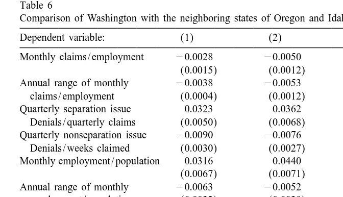
As an alternative to the difference-in-differences models, we estimate spe-cifications that make use of the variation over time in average tax costs in Washington and its neighboring states. As was seen in Table 1, we were able to obtain the necessary information to calculate the average marginal tax cost since
35
1972 not only for Washington, but also for Oregon and Idaho. The variation of
these tax costs over time should lead to more precise estimates than were possible with the simple difference-in-differences estimator. Each of our outcome variables is regressed on the marginal tax cost in effect in the state at that time, state dummies and a variable equal to 1 if the observation comes from the 1985–1997 period. Parallel to the difference-in-differences estimates, some models include the interaction of state with the log of the monthly U.S. unemployment rate or with the log of the annual state unemployment rate. The standard errors are calculated allowing for correlation within each of the six groups defined by the interaction of the three states with two time periods (pre-1985, post-1984).
Table 6 presents the results from this exercise. Recall that since the change in
34
For example, only Rhode Island, Delaware, Maine and West Virginia experienced larger drops in the range of annual claims than did Washington.
35
Table 6
a Comparison of Washington with the neighboring states of Oregon and Idaho
Dependent variable: (1) (2) (3)
Monthly claims / employment 20.0028 20.0050 20.0026
(0.0015) (0.0012) (0.0009)
Annual range of monthly 20.0038 20.0053 20.0068 claims / employment (0.0004) (0.0012) (0.0022) Quarterly separation issue 0.0323 0.0362 0.0348
Denials / quarterly claims (0.0050) (0.0068) (0.0060) Quarterly nonseparation issue 20.0090 20.0076 20.0074
Denials / weeks claimed (0.0030) (0.0027) (0.0030) Monthly employment / population 0.0316 0.0440 0.0410
(0.0067) (0.0071) (0.0051)
Annual range of monthly 20.0063 20.0052 20.0115 employment / population (0.0032) (0.0030) (0.0039)
Monthly Ln(employment) 0.1726 0.1994 0.2253
(0.0269) (0.0391) (0.0535)
Annual range of monthly 20.0110 20.0114 20.0197
Ln(employment) (0.0049) (0.0051) (0.0077)
Additional controls None State*ln(US UR) State*ln(state UR) a
Notes: Each reported coefficient comes from a separate regression of the dependent variable on the average marginal tax cost in the state at that time. All models also include state dummies and an indicator for the 1985–1997 period. Additional controls are included as indicated. Standard errors are in parentheses and are corrected for correlation within state and period.
the average marginal tax cost in Washington after the move to experience rating was approximately 1, the magnitude of the coefficient here should be similar to that from the difference-in-differences estimates of Table 5. Across all models, the point estimates for the key UI claim rate regression are quite similar to those from Table 5. In this case, however, the additional time-series variation leads to results
36
that are statistically significant at conventional levels. Looking at model (3), for
example, the point estimate of 20.0026 implies a 7.6 percent decline relative to
the claim rate in Washington before the implementation of experience rating, compared to the 10 percent drop implied by the analogous difference-in-differ-ences model. Similarly, this model implies a 31 percent drop in the range of the claim rate, about the same as the 29 percent decline from the estimate in Table 5. Results are also similar across methods for the other UI program variable for which the theory is most clear, the separation denial rate. The positive effect of experience rating on separation denials is significant and similar in magnitude to that estimated from the difference-in-differences models, with model (3) implying a 67 percent increase, compared to 56 percent in Table 5.
The point estimates for the nonseparation denials, however, are quite a bit more
36
negative than those obtained previously, with model (3) implying a 45 percent drop compared to only a 9 percent fall using the difference-in-differences estimate. The same is true for the range of employment measures. For example, looking at the range of log employment, a 29 percent drop is implied here by model (3), but only an 11 percent decline is found in Table 5. Similarly, the log of employment and employment / population ratio models led to uniformly more positive point estimates. In this case, model (3) implies a 7 percent increase in the employment / population ratio, compared with a 9 percent decrease in the corresponding difference-in-differences model. In general, though, for those outcome variables most tightly linked to theory, experience rating is estimated to have an impact similar to that found in Table 5, adding weight to the conclusion that experience rating has important effects on labor market and UI program outcomes.
6. Conclusions
A natural setting to examine the effects of the unemployment insurance payroll tax on wages, employment, UI claims and denials is provided by the recent experience of Washington State. Federal legislation forced Washington to adopt an experience rated system, beginning in 1985. After 13 years in which all employers paid the same UI tax rate, employers faced a wide range of tax rates, with each firm’s tax rate a function of its past use of UI. Thus, a comparison of wages and UI program and labor market outcomes before and after the change has the potential to provide good evidence on both tax incidence and the effects of experience rating.
To examine the incidence of the UI tax, we use individual level administrative earnings data. Our results are broadly supportive of the predictions of the models we propose. Labor earnings always fall with higher taxes. In our preferred specifications, we find evidence that the market-level tax is largely passed on to the worker in the form of lower earnings. Further, these estimates generally indicate that the firm can shift very little of the firm-level tax. This result implies that a country making the move to an experience-rated system might see a substantial reallocation of labor across firms, even though very little overall employment loss would be expected. Such reallocation may be appropriate in the case of UI, since without experience rating, high layoff firms are subsidized by more stable firms. Of course, for the case of using variable tax rates to finance other programs and mandates, such reallocation may imply deadweight losses.
the level and seasonality of claims fell, as did the seasonality of employment. While the expected effect on employment levels is theoretically ambiguous, we obtain some significant coefficients. Specifically, we find some evidence that the employment level rose. However, the employment effects seem too large and are only present in some of the specifications, inclining us to discount these results. Our estimates imply that a country contemplating a move to full experience rating might expect UI claim rates to fall between 10 and 33 percent, and the seasonality of this rate to fall 16–40 percent. Similarly, a drop of about 11 percent in the seasonal range of employment would be predicted. These results clearly suggest that experience rating reduces UI claims and stabilizes employment. Both of these changes mean lower unemployment and, thus, likely higher social welfare.
In terms of the effect of experience rating on employers’ involvement in the administration of benefits, we find strong evidence of an added incentive to ‘‘police the system’’ and contest invalid claims. Our results imply that experience rating increases the frequency with which UI claims are contested by employers. In Washington State, separation denials rose by 51–66 percent after the move to an experience rated system. We are unable, however, to gauge whether such an increase in denials is desirable on a cost-benefit basis. Finally, while we did not have definite predictions for nonseparation issue denials, we find some evidence of a fall.
Acknowledgements
We thank Janet Currie, Roger Gordon, Thomas Lemieux, two anonymous referees, and participants at the TAPES conference in Copenhagen in May 1998 for their comments and Brian Jenn and Dan Rosenbaum for excellent research assistance. We thank Cindy Ambler at the Department of Labor and Wayne McMahon and Hao Duong of Washington State Employment Security for providing data. The initial work on this project was funded under Purchase Order No. M-5110-5-00-97-40 from the U.S. Department of Labor, Advisory Council on Unemployment Compensation. The opinions stated in this document do not necessarily represent the official position or policy of the U.S. Department of Labor, Advisory Council on Unemployment Compensation.
Appendix A. Tax costs under experience rating in Idaho, Oregon and Washington
This appendix describes how we calculate the average marginal tax costs for
37
Idaho, Oregon and Washington over the 1972–1997 period. Both Oregon and
37
Washington have benefit ratio experience rating systems. In a benefit ratio system, the tax rate is an increasing function of the benefit ratio. This ratio is defined to be the average annual benefits charged to a firm over a period of years, divided by the average taxable payroll over the same period. Oregon uses a three year period, while Washington uses four years. The tax rate that a firm pays rises in steps as this benefit ratio increases. In both states the beginning and ending ratios for each of the steps (tax rates) are calculated so that specified percentages of taxable payroll fall in each tax bracket.
To calculate the tax cost, e, under this system we follow Topel (1990), and use the following formula:
2T
(12(11i ) )
]]]]]
e5h (A.1)
Ti
whereh is the slope of the schedule, i is the nominal interest rate, and T is the
number of years averaged. Using this formula and the fact that T54 in
Washington, and setting i50.1 we calculate that e50.79h for Washington.
Similarly, e50.83h for Oregon.
Idaho has a reserve ratio experience rating system that makes the tax rate a decreasing function of the reserve ratio. This ratio is defined to be the cumulative sum of all past years’ tax payments minus the cumulative sum of all past years’ benefit charges, all divided by the average taxable payroll over a recent period. The tax rate that a firm pays falls in steps as this reserve ratio increases. As in Oregon and Washington, the beginning and ending ratios for each of the steps are calculated so that specified percentages of taxable payroll fall in each tax bracket. To calculate the tax cost in Idaho, we use the formula derived in the appendix to Anderson and Meyer (1994):
2
g h ]]]
e5 2 , (A.2)
g h 1i
whereg is the growth factor for taxable wages, i.e. one plus the growth rate of
taxable wages. We calculateg as the average over the 1972–1997 period.
To obtain the average marginal tax cost for each state and year we average the tax costs in each tax bracket, weighting by the fraction of taxable payroll that is assigned to each bracket. We take the tax cost to be zero at the minimum and maximum rates because even non-marginal changes in benefit or reserve ratios at these extremes may result in no tax change. In all states the tax schedule is actually a step function rather than a differentiable function. To calculate the slope
h we average the height of a step up and a step down (the change in the tax rate)
separately for firms with positive and negative reserve ratios. To obtain overall percentages of payroll we used the average negative balance (reserve ratio) fraction over the 1983–1998 period.
References
Aaron, H.J., Bosworth, B.P., 1994. Economic issues in reform of health care financing. Brookings Papers on Economic Activity: Microeconomics, 249–299.
Advisory Council on Unemployment Compensation, 1995. Unemployment insurance in the United States: benefits, financing, and coverage. Washington, DC.
Anderson, P.M., 1993. Linear adjustment costs and seasonal labor demand: evidence from retail trade firms. Quarterly Journal of Economics 108, 1015–1042.
Anderson, P.M., Meyer, B.D., 1993. The Unemployment Insurance Payroll Tax and Interindustry and Interfirm Subsidies. In: James Poterba (Ed.), Tax Policy and the Economy 7, M.I.T. Press, Cambridge.
Anderson, P.M., Meyer, B.D., 1994. The effect of unemployment insurance taxes and benefits on layoffs using firm and individual data. National Bureau of Economic Research, Working Paper No. 4960.
Anderson, P.M., Meyer, B.D., 1997. The effects of firm specific taxes and government mandates with an application to the U.S. unemployment insurance program. Journal of Public Economics 65, 119–145.
Ashenfelter, O., Levine, P.B., 1996. Unemployment insurance appeals in the state of Wisconsin: who fights and who wins? Advisory Council on Unemployment Compensation: Background Papers Volume IV. Washington, DC.
Becker, J.M., 1972. Experience Rating in Unemployment Insurance: an Experiment in Competitive Socialism. The Johns Hopkins University Press, Baltimore.
Becker, J.M., 1981. Unemployment Insurance Financing: an Evaluation. American Enterprise Institute, Washington.
Card, D., Levine, P.B., 1994. Unemployment insurance taxes and the cyclical and seasonal properties of unemployment. Journal of Public Economics 53, 1–29.
Gruber, J., 1994. The incidence of mandated maternity benefits. American Economic Review 84 (3), 622–641.
Gruber, J., 1995. The incidence of payroll taxation: evidence from Chile. NBER Working Paper No. 5053.
Gruber, J., Krueger, A., 1991. The incidence of mandated employer-provided insurance: lessons from workers’ compensation insurance. In: Bradford, D. (Ed.), Tax Policy and the Economy. NBER, Cambridge, pp. 111–143.
Hamermesh, D.S., 1993. Labor Demand. Princeton University Press, Princeton, NJ.
Levy, F., Murnane, R.J., 1992. U.S. earnings levels and earnings inequality: a review of recent trends and proposed explanations. Journal of Economic Literature XXX, 1333–1381.
Meyer, B.D., 1995. Natural and quasi-experiments in economics. Journal of Business & Economic Statistics 13, 151–162.
Munts, R.C., Asher, E., 1981. Cross-Subsidies Among Industries From 1969 to 1978. National Commission on Unemployment Compensation, Unemployment Compensation: Studies and Re-search, Washington, D.C.
Nickell, S., 1986. Dynamic models of labour demand. In: Ashenfelter, O., Layard, R. (Eds.), Handbook of Labor Economics. North Holland Press, Amsterdam.
Topel, R.H., 1990. Financing unemployment insurance: history, incentives, and reform. In: Hansen, W.L., Byers, J.F. (Eds.), Unemployment Insurance. University of Wisconsin Press, Madison, Wisconsin.
Vroman, W., 1996. Disputes over unemployment insurance claims: a preliminary analysis. Advisory Council on Unemployment Compensation: Background Papers Volume IV. Washington, DC. Washington State Employment Security, 1984. Experience rating: unemployment insurance tax
information for Washington state employers. Olympia, Washington, Unemployment Insurance Division.
Washington State Employment Security, undated (a). Major legislative changes in benefit provisions at a glance. Unemployment Insurance Division, Olympia, Washington.