Full Terms & Conditions of access and use can be found at
http://www.tandfonline.com/action/journalInformation?journalCode=ubes20
Download by: [Universitas Maritim Raja Ali Haji] Date: 12 January 2016, At: 17:48
Journal of Business & Economic Statistics
ISSN: 0735-0015 (Print) 1537-2707 (Online) Journal homepage: http://www.tandfonline.com/loi/ubes20
Cromwell's Rule and the Role of the Prior in the
Economic Metric
Kenneth D Roskelley
To cite this article: Kenneth D Roskelley (2008) Cromwell's Rule and the Role of the Prior in the Economic Metric, Journal of Business & Economic Statistics, 26:2, 227-236, DOI: 10.1198/073500107000000160
To link to this article: http://dx.doi.org/10.1198/073500107000000160
Published online: 01 Jan 2012.
Submit your article to this journal
Article views: 44
Cromwell’s Rule and the Role of the Prior in
the Economic Metric: An Application to
the Portfolio Allocation Problem
Kenneth D. R
OSKELLEYDepartment of Economics and Finance, Louisiana Tech University, Ruston, LA 71272 (kennethr@latech.edu)
We show that using Bayesian decision theory to draw inference about the economic significance of a model requires careful specification of model uncertainty in the prior density. As an example, we use the Bayesian investor’s portfolio allocation problem to show that failure to include probability point mass on the null hypothesis that returns are not predictable will overstate the economic significance of the predic-tive model. The dissonance between the statistical and economic significance of asset return predictability seen in previous research appears to be an artifact of how model uncertainty is treated in the specification of the prior.
KEY WORDS: Bayesian econometrics; Model uncertainty; Point-null hypothesis; Variable selection.
“I beseech you, in the bowels of Christ, think it possible you may be mistaken.” Letter from Oliver Cromwell to the General Assembly of the Scottish Kirk, August 3, 1650.
1. INTRODUCTION
Bayesian decision theory is a useful tool in quantifying the economic, as opposed to statistical, significance of models and variables. Although inference can differ across the two metrics, they tend to be related to each other. One aspect of hypothe-sis testing that is occasionally absent in studies that focus on the economic metric is the presence of two models, a null and an alternative hypothesis. The lack of competing models can inadvertently drive a wedge between the perceived economic and statistical significance of a model and is a violation of what Poirier (1988) calls Cromwell’s rule: Never assign probability of 1 to any model. In such a framework, it is inappropriate to draw inference about the economic significance of a model un-less there exists absolutely no uncertainty about the model’s va-lidity. To illustrate this point, we use the economic metric of asset return predictability proposed by Kandel and Stambaugh (1996) to show that including a model to represent a point null hypothesis can greatly change the model’s perceived economic value.
In particular, we document that the strong evidence that asset returns are predictable (Kandel and Stambaugh 1996) is in fact due not to the use of an economic as opposed to a statistical loss function, but rather to the choice of the investor’s prior. We show that even though the model of no predictability is spanned by the parameter space of the linear predictive regression, using a continuous prior over the regression’s parameter space does not result in a prior that encompasses both models. Because the model of no predictability is a point-null hypothesis (i.e., the slope parameters equal 0), using a continuous prior over the regression parameters places all of the probability mass on the model of predictability. As a result, placing a small amount of point mass at 0 in the investor’s prior to represent a point null hypothesis can lead to very different economic inference than when the investor’s uncertainty about the predictive regression is represented solely by a continuous prior over the parameter space.
Although Kandel and Stambaugh (1996) argued that the pa-rameter estimates in the posterior should bunch up around 0 if returns are not predictable, such an approach does not allow for an analysis of the relative strength of evidence in the data that returns are predictable versus unpredictable. This methodology violates Bayesian principals for hypothesis testing and decision analysis when model uncertainty exists (see Robert 2001 for a more detailed discussion). An example illustrates this point. Consider an investor that attempts to allocate his or her wealth between a risky and a risk-free asset to maximize his or her ex-pected utility. To do so, he or she must form a prediction about next period’s return on the risky asset. Assume that he or she knows that 1% of all variables are able to predict the future risky return and that the probability that a predictive variable will be statistically significant when analyzed is 99%. The investor also knows that there is only a 1% probability that a nonpredictive variable will be found to be statistically significant. However, due to the ratio of predictive to nonpredictive variables in the data, Bayes’s rule implies that only half of all variables found to be statistically significant will in fact be predictive variables. Thus if the investor finds a variable that predicts returns in the historical data, then he or she should form his or her forecast about next period’s return as the average between the uncon-ditional historical return and the conuncon-ditional return indicated by the predictive variable. Nevertheless, if the investor has no point mass in the prior at 0 (as in Kandel and Stambaugh 1996), then he or she cannot evaluate Bayes’s rule, because all of the probability mass in the prior (and thus posterior) lies under the model of predictability. As a result, the investor will form his or her beliefs about future returns based entirely on the predic-tive variable and will not be able to optimize his or her portfolio allocation over both type I and type II errors.
To show that it is the investor’s prior that drives the disso-nance between economic and statistical inference reported by Kandel and Stambaugh (1996), we recast the portfolio alloca-tion problem to allow for a point-null hypothesis that the re-gression’s slope parameters are 0. First, we place point mass in
© 2008 American Statistical Association Journal of Business & Economic Statistics April 2008, Vol. 26, No. 2 DOI 10.1198/073500107000000160 227
the investor’s prior that all of the slope coefficients in the pre-dictive regression are jointly 0, and then show that the resulting economic inference mirrors that of a classicalF test. Second, we place point mass in the prior that any individual slope coef-ficient is 0. This allows the investor to place different weights on the different predictive variables when forecasting returns, and the resulting economic inference is similar to a maximal
tstatistic test.
The goal of this article, however, is not to prove or disprove the existence of predictability in returns, or to analyze the ques-tion of optimal forecasting. Rather, the aim is to investigate the sensitivity of the economic metric to the choice of a prior when the model is not known with certainty. To focus on the role of the prior in the metric of economic significance and abstract away from other econometric problems such as unit roots (see Stambaugh 1999; Torous, Valkanov, and Yan 2004; Campbell and Yogo 2005), we use simulated data calibrated to historical U.S. data in conjunction with the historical returns on a value weighted portfolio of the stocks traded on the New York Stock Exchange.
The article is organized as follows. Section 2 provides an overview of related literature, whereas Section 3 reviews the portfolio allocation problem of Kandel and Stambaugh (1996) when the model of predictability is known. The framework is then extended to an allocation problem where the investor’s prior over the regression parameters includes point mass at 0. Section 4 explores the effect of placing point mass in the prior on a variable’s economic significance. Section 5 contains a summary of the results and some concluding remarks.
2. LITERATURE REVIEW
Despite the growing sentiment that returns are predictable, several studies provide caveats about interpreting the statisti-cal results. Richardson (1993), for instance, pointed out the lack of power in many statistical tests, whereas Foster, Smith, and Whaley (1997), White (2000), Sullivan, Timmermann, and White (2001), and Ferson, Sarkissian, and Simin (2003) pointed out that the presence of data snooping makes it difficult to inter-pret the statistical significance of the variables. More closely re-lated to this article is the work of Lamoureux and Zhou (1996), which showed that a diffuse prior over the parameters does not necessarily result in a diffuse prior over a function of those pa-rameters, which can in turn lead tests like the variance ratio to overstate the evidence of predictability in the data.
Kandel and Stambaugh (1996) sought to avoid these statis-tical problems by instead focusing on the variable’s economic importance. To do so, they measured the predictability of re-turns by looking at how a risk-averse Bayesian investor would use the data in allocating wealth between a risk-free asset and a risky asset. Surprisingly, Kandel and Stambaugh found that even for cases where there is no statistical evidence of pre-dictability, the investor makes appreciable changes in his or her portfolio allocation between the risky asset and risk-free asset based on the data. One possible conclusion from their analy-sis is that despite data mining concerns and the lowR2 typi-cally found in the literature, representative investors from asset pricing models would find the degree of predictability in ac-tual historical returns significant enough to alter their portfolio allocations.
Following Kandel and Stambaugh (1996), other studies have also focused on the portfolio allocation problem. Pastor (2000), Pastor and Stambaugh (2000), and Brennan and Xia (2001) all looked at the effect of uncertainty on an investor’s portfolio al-location. They focused on portfolio choices for investors who are uncertain of the validity of risk-based versus characteristic-based asset pricing models. Tu and Zhou (2004) expanded the analysis to include uncertainty over the distributional form of the data-generating process. Although these authors examined the economic evidence associated with asset pricing anomalies, they did not focus on the sensitivity of the economic metric to the specification of the prior over the model space.
Closely related to this study’s treatment of the investor’s prior beliefs are Avramov (2002) and Cremers (2002), who use the context of optimal forecasting to illustrate the superiority of Bayesian model averaging to classical model selection crite-ria. Although their methodology is similar to our own, neither paper investigates the sensitivity of the economic metric to the specification of the prior. Cremers (2002), for instance, used 14 variables to forecast the S&P 500 and found that the pos-terior probabilities are generally supportive of predictability in returns. Cremers (2002) also showed that the Bayesian model-averaged forecast outperforms classical model selection crite-ria, in general exhibiting lower mean squared error and bias.
Avramov (2002), on the other hand, used 14 regressors to ex-amine portfolio returns sorted according to size and market to book and forecast the returns on the CRSP value-weighted in-dex. Like Cremers (2002), he also showed that posterior odds ratios tend to support predictability and that Bayesian model averaging outperforms classical model selection criteria in out-of-sample forecasting. Avramov (2002) also used one set of re-gressor values to demonstrate that the portfolio allocation prob-lem is more sensitive to regressor uncertainty than to parameter uncertainty. Similarly, he showed that there can be a substantial utility gain for an investor who uses Bayesian model averag-ing instead of classical model selection criteria. However, he did not investigate the economic significance of predictability in the data by comparing the utility gain of using the uncondi-tional mean (iid returns model) with the optimal forecast given by Bayesian model averaging.
3. PORTFOLIO ALLOCATION: THE METRIC OF ECONOMIC SIGNIFICANCE
Consider a risk-averse investor with a one-period investment horizon whose preferences are represented by the power utility function, defined as
v(WT+1)=
1
1−AW
1−A
T forA>0,A=1 lnWT forA=1,
whereWT is the investor’s wealth at the end of time period
T andA represents the investor’s degree of risk aversion. At the end of time periodT, the investor must allocate his or her wealth,WT, between a risky asset and a risk-free asset. The in-vestor’s wealth at the end of time periodT+1 is then written as
WT+1=WT[ωerT+1+iT+1+(1−ω)eiT+1], 0≤ω <1, whereiT+1is the return on the risk-free asset,rT+1is the
con-tinuously compounded excess return on the risky asset, andωis
Roskelley: Role of Prior in Portfolio Allocation Problem 229
the percentage of wealth that the investor allocated to the risky asset at the end of time periodT.
Furthermore, assume that the investor at the end of timeT
also observesT=(r1, . . . ,rT,X0, . . . ,XT−1,XT), wherert+1
is the observed return at timet+1 andXtis ak+1 vector con-taining a scalar andkeconomic variables observed at timetthat are thought to predictrt+1. The investor uses this historical data
to estimate the following predictive model for stock returns:
rt+1=XtTβ+ǫt+1, (1)
whereβ is a vector with an intercept coefficient andk slope coefficients andǫt+1is a mean-0, normally distributed random
variable with varianceσ2. Instead of rejecting or failing to re-ject a hypothesis about the predictability of returns, the investor uses the information inT to formp(rT+1|T), his or her con-ditional belief about the distribution of returns for time period
(T+1). Combining the investor’s utility function,v, with the predictive density for returns,p(rT+1|T), gives an expected utility maximization problem of the form
max
0≤ω<1
v(WT+1)p(rT+1|T)drT+1. (2)
3.1 The Kandel–Stambaugh Framework
Following the exposition of Zellner (1971) and Kandel and Stambaugh (1996; hereinafter referred to simply as KS), the investor formsp(rT+1|T)by first using the historical data to update his or her prior beliefs about the predictive model’s pa-rametersβ andσ. The posterior distribution of the parameters,
p(β, σ|T, ), may be expressed as being proportional to the product of the investor’s prior beliefs and the model’s likeli-hood,
p(β, σ|T, )∝p(β|σ )·p(σ )·p(T|β, σ ),
wherep(T|β, σ ) is the likelihood defined by the predictive regression of equation (1). This posterior density on the para-meters is then combined with the predictive likelihood for equa-tion (1) to obtain the joint density for the parameters and future returns,
p(rT+1, β, σ|T)=p(β, σ|T)·p(rT+1|β, σ,XT). Integrating over the unknown parameters β and σ gives
p(rT+1|T), the conditional predictive density for next month’s return,rT+1,
p(rT+1|T)= p(rT+1, β, σ|T)dβdσ. (3)
The investor then maximizes his or her expected utility [eq. (2)], by choosing the percent of his or her wealth,ω, to invest in the risky asset. To measure the predictability in returns, a compari-son is made between the portfolio allocation of an investor that uses the predictive regression model in forming p(rT+1|T) and one that uses the unconditional mean of the historical data. As an example, KS examined the portfolio allocation of an investor with a risk-aversion parameter ofA=2. They reported that such an investor would put 94% of his or her wealth in the risky asset if he or she used the iid model in forming his or her beliefs about the time(T+1)return given that he or she had observed 67 years of historical returns with an average monthly
excess return of .49% and a standard deviation of 5.6%. KS then compared this unconditional portfolio allocation with that of an investor who used the conditional return from a predictive regression with an R2 of 2.5% that liesδ regression standard deviations from the unconditional mean, or when
rT+1=r+δσr
R2, (4)
whererT+1represents the expected return for time(T+1)
con-ditional onXT,ris the average return over the 67-year sample, andσris the return’s sample standard deviation.
KS reported that the investor would completely divest him-self or herhim-self of the risky asset if the conditional return at time
(T+1)were one regression standard deviation below the sam-ple mean(δ= −1). This would be true even if the predictive regression included 25 variables. This seems to suggest that, despite apvalue of about 75% for the regression, an investor nonetheless would reject the hypothesis that stock returns are not predictable by significantly reweighting his or her portfo-lio. KS further showed that Bayesian odds ratios and frequen-tist pvalues lead to similar statistical inference, leaving them to conclude that the difference in inference is due to the use of an economic as opposed to a statistical loss function. They in-ferred that p values are poor indicators of the strength of the evidence in the data against the null hypothesis that returns are not predictable.
3.2 Portfolio Allocation With Point Mass in the Prior
Note that, unlike in classical statistical inference, in the KS framework no comparison is made between the null and alter-native hypotheses. Thus the investor cannot weigh the strength of the evidence against the predictive regression. The investor instead believes with certainty that the predictive regression is an accurate description of the return-generating process, be-cause no probability mass is placed in his or her prior on the null hypothesis. Such an approach avoids the accept–reject de-cision made in classical statistical tests by instead focusing on how an investor would use the information in allocating his or her wealth between assets. But the weakness of this approach is that the investor is not allowed to adjust his or her decision based on his or her uncertainty about what is the optimal model for solving the portfolio allocation problem. The lack of prob-ability mass on alternative models makes it impossible for the investor to make a probabilistic statement about which regres-sors are predictive, or if in fact the model ofnopredictability is not more realistic than any of the predictive regression models. This precludes the investor from making the portfolio allocation decision while optimizing over type I and type II errors.
There are two obvious ways to introduce uncertainty into the investor’s prior that mimic classical statistics. The first is to compare the predictive regression to the unconditional mean, as in anF statistic. This may be done by including point mass in the investor’s prior that all of the slope coefficients are si-multaneously equal to 0 and will allow the investor to gauge the relative merits of the predictive regression model to the iid model. The second method is to focus on the significance of each individual regressor, as in atstatistic. This may be done (as in Cremers 2002; Avramov 2002) by placing point mass in the investor’s prior that individual slope coefficients are 0. (See
Madigan and York 1995; Chen, Shao, and Ibrahim 2000 for a more detailed theoretical analysis.) Thus the investor’s predic-tive density p(rT+1|T) is a probability-weighted average of the 2kcandidate models represented by different combinations of those regressors, including the model that returns are not pre-dictable (iid).
In either case, let I represent the total number of models that the investor entertains, and letMi represent theith model. The investor’s conditional density for returns is calculated as a probability-weighted average over theIconditional densities for returns, or The marginal densities for each model can be considered a weighted average of the likelihood, with the weights given by the prior density on the model’s parameters. Details on how the posterior densityp(rT+1|T)is calculated numerically and used to maximize the investor’s expected utility function are given in the Appendix.
For consistency with KS, assume that the investor’s prior be-liefs about modelM′isslope parameters and intercept,p(βi|σi,
Mi), may be accurately described as a multivariate normal dis-tribution,βi∼N[βi, i], whereas the prior distribution forσi,
p(σi|Mi), is given byviσ2/σi2∼χ2[υi]. Let thekiprior means on the slope parameters found inβ
ibe set to 0, and let the mean of the intercept parameter equal the historical average of re-turns. In addition, let the prior mean σ2i equal the variance of historical returns,σr2, and the degrees of freedom,vi, equal the number of hypothetical observations,T0, minus the number of
parameters inβi,ki+1. To maintain the general structure of the observed data in the prior density, leti=(TT
0 T
ii)−1, where
Ti is the(ki+1)×T matrix containing a column of 1’s and the T historical observations on the ki regressors included in modelMi. HereTii is multiplied by TT
0, the ratio of the ob-served sample size to the degrees of freedom of the prior distri-bution, so that a more informative prior, as given by a largerT0,
will have a smaller covariance matrix while still matching the sample properties of the observed data. (See Zellner 1986 for more details on using sample information in the specification of the prior.) As KS pointed out, this prior is meant to represent
T0hypothetical observations in a regression that has anR2of 0.
Whereas KS also used a noninformative prior in their analy-sis, as Lindley (1957) pointed out, it is not possible to calculate posterior probabilities over the models when the prior is not a proper density. To minimize the effect of the prior on the port-folio allocation, the investor’s prior beliefs in this article will representT0=50+ki+1 hypothetical monthly observations.
4. RESULTS
To illustrate the role of the prior in driving a wedge between the economic and statistical metrics, we break down the analy-sis into two sections. In the first section the investor’s posterior belief about the next period’s return is a weighted average be-tween only two models: the unconditional return and the predic-tive regression model defined by allkvariables. This analysis is similar to classical inference using anFstatistic and is accom-plished by placing point mass that all of the slope parameters are simultaneously equal to 0. The portfolio weights for this in-vestor are then compared with the KS case in which the inin-vestor uses only the predictive regression in formingp(rT+1|T). In the second section the investor’s prior includes point mass at 0 for each individual regressor in the composite model. Here the analysis is similar to classical inference using a maximalt sta-tistic, and the investor makes his or her allocation decision by averaging over the 2k candidate models that can be formed by thekregressors. Once again, the optimal portfolio weights for this investor are then compared with the KS baseline case.
4.1 Data Set
The predictive regression used in this article includes five variables previously analyzed for their ability to predict mar-ket returns: dividend yield, dividend growth, the spreads of Aaa bonds and Bbb bonds over the 1-month Treasury rate, and the difference between the 1-month T Bill and its 1-year moving average. These five variables are used in the following linear regression to predict the excess monthly return of the value weighted portfolio of stocks listed on the New York Stock Ex-change:
Excess returnt+1
=α+β1dividend yieldt+β2dividend growth ratet
+β3Baa spreadt+β4Aaa spreadt
+β51-month T-Bill minus 1-year moving averaget+εt. The data consist of 708 monthly observations from between January 1934 and December 1993, and the regression’sR2is 4.9%. The dividend and return data are taken from CRSP, the Treasury data are obtained from Ibbotson Associates (1997), and corporate bond data are collected from the St. Louis Fed-eral Reserve. The regression results, along with descriptive sta-tistics, are reported in Table 1.
Because the goal of the analysis is to understand the role of model uncertainty and size as specified in the investor’s prior, these five predictive regressors are jointly used with simulated data to evaluate the investor’s portfolio allocation. The use of simulated data avoids the introduction of ancillary econometric issues such as unit roots, multicollinearity, and endogeneity as the size of the predictive regression increases. Each of the simu-lated variables is constructed by matching the first two moments of a normal density to one of the economic variables given in Table 2. Because the structure of the simulated data may in-fluence inference through the calculation of the marginal like-lihoods for the data (see Koop 2003; Zellner 1971), we repeat the analysis in all sections of this article on different simulated data sets. Although there are small differences in the portfolio allocations for the different data sets, the qualitative results re-ported here appear to be robust to these concerns.
Roskelley: Role of Prior in Portfolio Allocation Problem 231
Table 1. Predictive regression of monthly NYSE index returns
Coefficient T-statistic Sample mean Sampleσ
Intercept −.0104 −1.70
NOTE: This table reports the results of regressing the 1-month excess return from a value weighted portfolio of NYSE stocks onto five predictive variables. Dividend yield is the sum of all dividends for NYSE stocks paid over the last year divided by the current sum of the prices. Dividend growth is the growth in the dividend yield over the previous month. Aaa spread is the spread between Aaa bonds and the 1-month T-Bill. Baa Spread is the spread between Baa bonds and the month T-Bill. T-Bill MA is the difference between the 1-month T-Bill and its 1-year moving average. NYSE return and dividend information are obtained from CRSP. T-Bill data are obtained from Ibbotson Associates (1997). Corporate bond data are obtained from the St. Louis Federal Reserve. The data begin in January 1935 and end in December 1993.
4.2 Optimal Portfolio Weights
Two Models. In this section we explore how the economic significance of predictability is affected when the investor is allowed to place point mass in his or her prior that the slope parameters in the predictive regression are jointly equal to 0. This prior specification leads to inference similar to that of an
Fstatistic and allows the investor to analyze the data through two competing models: the predictive regression and the uncon-ditional mean. To bias the results against finding a reversal in economic significance when model uncertainty is introduced, we set the investor’s risk aversion parameter to 5 (A=5) and let the investor’s prior probability on the model of predictability equal 90%. In addition, whereas KS used a VAR model to alle-viate concerns about endogeneity, we use a standard regression model to further bias the results against finding a reduction in economic significance.
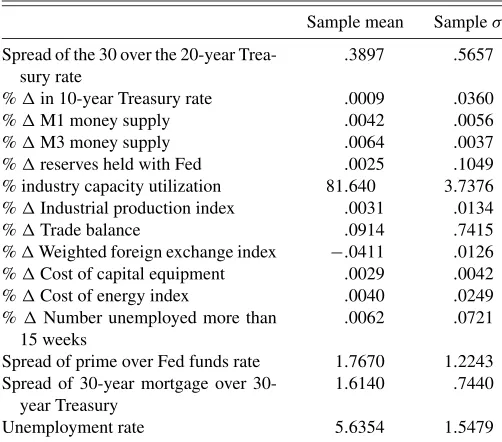
Table 2. Descriptive statistics of the auxiliary data set
Sample mean Sampleσ
Spread of the 30 over the 20-year Trea-sury rate
% industry capacity utilization 81.640 3.7376
%Industrial production index .0031 .0134
%Trade balance .0914 .7415
%Weighted foreign exchange index −.0411 .0126
%Cost of capital equipment .0029 .0042
%Cost of energy index .0040 .0249
%Number unemployed more than
15 weeks
.0062 .0721
Spread of prime over Fed funds rate 1.7670 1.2243
Spread of year mortgage over 30-year Treasury
1.6140 .7440
Unemployment rate 5.6354 1.5479
NOTE: This table reports descriptive statistics for the 15 variables used in calibrating the simulated data. The simulated variables are based on the first and second moments of the historical monthly observations reported by the St. Louis Federal Reserve.
Following the exposition of KS, and to explore the sensitivity of the economic metric to model size, we first analyze the op-timal portfolio allocation by fixing the predictive regression’s
R2and allowing the number of regressors to vary. To maintain theR2constant as the number of regressors increases, we use only simulated variables whenk>5. Each data set is formed by drawingkindependent and normally distributed variables until a data set that has an R2 within .1% of the original data’sR2
of 4.9% is obtained. The optimal portfolio allocation of an in-vestor that averages over the two models is then compared with that of the KS investor who considers only the predictive re-gression. This analysis makes it possible to examine the reward for parsimony in both frameworks conditional on the amount of variation explained by the predictive regression.
Table 3 presents the optimal portfolio allocation to the risky asset, ω, for an investor who uses k regressors to estimate
p(rT+1|T)given that the predictive regression’sR2 is 4.9%. Panel A contains the portfolio weights when the investor is as-sumed to know the model of predictability (as in KS), whereas panels B and C report the weights when the investor’s prior contains 10% and 50% point mass at 0. Note from panel A that when the investor uses the unconditional mean(δ=0)to allo-cate his or her wealth, he or she places 64.7% in the risky asset. On the other hand, if he or she observed anXT containing five predictive variables(k=5)with an expected future return that is one regression standard deviation below the unconditional mean (δ= −1), then he or she would invest nothing in the risky asset. Furthermore, had the investor obtained the R2 of 4.9% from a regression of 60 variables(k=60), then his or her al-location to the risky asset would still be 0. Despite the fact that
Table 3. Optimal portfolio weights whenR2is 4.9%
k δ= −1 δ= −.5 δ=0 δ=.5 δ=1
A: No probability mass at 0 in the investor’s prior
5 0% 20.7% 64.7% 99.9% 99.9%
15 0% 21.0% 64.7% 99.9% 99.9%
30 0% 21.7% 64.7% 99.9% 99.9%
45 0% 22.4% 64.7% 99.9% 99.9%
60 0% 23.0% 64.7% 99.9% 99.9%
B: 10% probability mass at 0 in the investor’s prior
5 0% 20.8% 64.7% 99.9% 99.9%
15 0% 21.1% 64.7% 99.9% 99.9%
30 1.4% 32.3% 64.7% 98.8% 99.9%
45 63.2% 64.0% 64.7% 65.4% 66.0%
60 64.7% 64.7% 64.7% 64.7% 64.7%
C: 50% probability mass at 0 in the investor’s prior
5 0% 21.0% 64.7% 99.9% 99.9%
15 0% 21.8% 64.7% 99.9% 99.9%
30 43.7% 54.0% 64.7% 74.7% 85.1%
45 64.5% 64.6% 64.7% 64.8% 64.9%
60 64.7% 64.7% 64.7% 64.7% 64.7%
NOTE: This table compares the optimal portfolio weight for the risky asset when the conditional mean from the predictive regression liesδregression standard deviations from the unconditional mean and there arekregressors. In panel A, the investor’s uncertainty about predictability is represented by centering the prior density at 0. In panels B and C, the investor’s uncertainty that returns are predictable includes placing point mass in her prior that the slope parameters are simultaneously equal to 0. In panel B, the investor places 10% of her subjective probability on the model that returns are not predictable (slopes equal 0), whereas in panel C the investor places 50% probability on the predictive regression. In all three cases, the investor’s prior beliefs about the regression’s slope parameters are centered at 0 and based on 50+k+1 hypothetical observations. Posterior beliefs are formed after observing 708 observations and estimating a predictive regression with anR2of 4.9%.
the regression with 60 variables is not statistically significant, the investor completely divests himself or herself of the risky asset, the same as in the case where there are only five regres-sors and the results are statistically significant.
This illustrates that the investor’s optimal portfolio allocation in the KS framework is insensitive to the number of regressors for a given level of explained variation. This means that the al-location decision also will be independent of the regression’s statistical significance, because there is no baseline model to which the predictive regression is compared. Panel B of Table 3 shows that this insensitivity to the number of regressors disap-pears once the investor is allowed to average over the model of predictability and the model of no predictability. Whereas the portfolio allocations seen in panels A and B are almost identi-cal for the case of 5 regressors, panel B shows that the portfolio allocations diverge as the number of regressors increases. The reason for this is that for a fixed R2, the amount of variation in returns explained by the regression is the same regardless of how many regressors are included in the predictive model. Hence, when the investor entertains no baseline model, her allo-cation decision is insensitive to the predictive regression’s size. Including point mass at 0 in the prior, on the other hand, allows the investor to weigh the relative merits of both the predictive regression and the iid model. This allows the posterior probabil-ities on the models, which themselves are closely related to the
Fstatistic as pointed out by Clyde and George (2004), to reflect the relative strength of the null and alternative hypotheses.
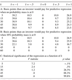
To quantify the economic significance in the data, KS calcu-late the difference, in basis points, between the investor’s cer-tainty equivalent utility under the conditional and unconditional means. This difference is interpreted as the amount that the in-vestor would be willing to give up for the information in the predictive regression. Table 4 compares the economic signifi-cance of the two portfolio allocation problems to the statistical significance. Panel A contains the basis points that the KS in-vestor would be willing to give up for the information in the predictive regression, and panel B lists the value to an investor that has point mass at 0 in his or her prior. Panel C reports the corresponding regression F statistics and p values. Note that from panels A and B, when theR2=4.9% andk=15, the in-vestors in both frameworks would pay approximately 39 basis points for the information that the conditional mean of the pre-dictive regression is one full regression standard deviation be-low its mean. Turning to panel C, thepvalue of this regression is .3%, so it is not surprising that both investors ascribe value to the predictive regression. But ifk=45, then the investor in the KS framework would still pay around 39 basis points (panel A), whereas the investor that takes model uncertainty into account would pay nothing (panel B). But adding these 30 variables in-creases the regression’sp value to 88.3%, indicating that the data favor the null over the alternative hypothesis.
This serves to illustrate that the divergence in inference be-tween the economic and statistical metrics seen in KS is forced by the absence of an alternative model. The KS framework overstates the evidence against the null hypothesis that returns are not predictable, because the null receives no probability mass in the investor’s prior. Indeed, comparing panels B and C shows that in fact thepvalues are good indicators of the eco-nomic information in the data when the investor is uncertain about the validity of the predictive regression.
Table 4. Economic and statistical significance of the predictive regression whenR2is 4.9%
k δ= −1 δ= −.5 δ=0 δ=.5 δ=1
A: Basis points than an investor would pay for predictive regression when no probability mass is at 0
5 39.2 10.5 0 10.0 26.9
15 39.0 10.4 0 9.7 25.9
30 38.9 10.1 0 9.3 25.2
45 38.8 9.9 0 8.9 24.3
60 38.5 9.7 0 8.5 23.5
B: Basis points than an investor would pay for predictive regression when 10% probability mass is at 0
5 39.2 10.5 0 10.0 26.9
15 38.6 10.3 0 9.4 25.9
30 22.1 5.8 0 4.8 16.7
45 0 0 0 0 0
60 0 0 0 0 0
C: Statistical significance of the regression as a function ofk
k Fstatistic pvalue
NOTE: This table reports the economic and statistical significance of the data. Panels A and B report the number of basis points an investor would be willing to give up to ob-tainXT, the vector containing the values of thekpredictive variables at timeT, to construct
the predictive density of future returns,p(rT+1|T). The value of the information to the
investor is listed as a function ofk, the number of variables, andδ, the number of regres-sion standard deviations the regresregres-sion forecast is above or below the unconditional mean. Panel A reports the value for an investor that places no probability point mass in her prior that the slope parameters are jointly 0, whereas in panel B the investor places 10% prob-ability mass at 0. Panel C reports both theFstatistic and thepvalue for the predictive regression as a function ofk, the number of regressors included, given that there are 708 observations and the regressionR2is 4.9%.
2k Models. Whereas the previous section analyzed the overall significance of the predictive model, this section focuses on the significance of the individual components of that model. Here the investor has point mass in his or her prior overβ that any individual regressor’s slope coefficient is 0 and thereby av-erages over the 2kmodels that can be formed with thek predic-tive regressors. This form of model uncertainty is similar to that of atstatistic and allows analysis of the economic significance of a variable conditional on the size of the original regression. Note that if the prior probability that a regressor is not useful in predicting future returns is set equal topfor allkvariables, then the investor’s prior probability on modelMican be written as
p(Mi)=(1−p)kipk−ki,
where ki represents the number of included regressors in modelMi. To maintain the implied subjective probability that returns are predictable at 10%, we setp=√k.1. This results in the sum of the prior probabilities on the 2k−1 predictive re-gressions equaling 90%, with 10% probability mass remaining on the iid model.
Unlike in the previous section, here theR2of the regression is allowed to change as simulated variables are added to the ac-tual data of Table 1. This analysis makes it possible to evaluate how model size influences the significance of individual regres-sors when the variation in the data explained by the variable is
Roskelley: Role of Prior in Portfolio Allocation Problem 233
held fixed. To augment the data set, we first add in 15 simu-lated variables to the original five. We do so 1,000 times to con-struct 1,000 data sets containing 20 regressors. We then keep only the data set corresponding to the medianR2. Next, we take this augmented data set and add in 20 more simulated variables and construct 1,000 more data sets, each containing 40 regres-sors. Once again, we keep only the data set corresponding to the medianR2. We repeat this last step until we have one data set containing a total of 141 variables—the original 5 regressors, the monthly excess returns on the NYSE value weighted aver-age, and 135 simulated variables. Note that in the analysis that follows that whenkincreases, the simulated variables are added in the order in which they were created. This means that when any two data sets are compared, the set with fewer regressors will always be a proper subset of the larger data set.
It is also important to note that in this section the choice of theXT used to define the regression standard deviation,δ, in-fluences the portfolio allocation. Whereas in the previous sec-tion the simulated variables influence the analysis only through computation of the Bayes factor, here the choice of XT also influences the computation of the conditional mean. That is, whereas different simulated values ofXTmay result in the same conditional mean for the composite model defined by allk vari-ables, in general those sameXT will result in different condi-tional means for the 2k−1 submodels because they do not in-clude all of the regressors inXT. Because the investor is taking a probability-weighted average over these conditional means, the choice ofXT will influence the results. Furthermore, because of the large number of draws needed to ensure convergence in the posterior askincreases in size, it is only feasible to solve the investor’s utility maximization problem and evaluate the port-folio allocation for a few values ofXT. In an attempt to mitigate these two problems, we formXT by analyzing all 708 obser-vations on thekpredictive variables and keeping each one that produces a conditional forecast for returns that is at least one regression standard deviation below the mean. We then keep the three observations that exhibit the largest deviations in the two variables that have the highest posterior probability. These six observations are then used asXT in separate maximization problems. All tables contain results for the simulated deviation that produces the largest movement in the investor’s optimal portfolio allocation. In most cases the reported optimal portfo-lio weights differ by only 1–2 percentage points, and in no case by more than 7.
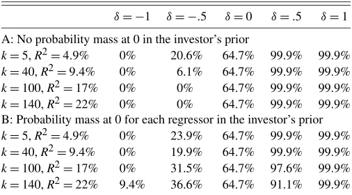
Table 5 reports the optimal portfolio weights as a function of the number of predictive regressors. Panel A shows the portfo-lio weights when the investor believes that he or she knows the model of predictability as in KS, whereas panel B shows the weights when the investor averages over the 2kcandidate mod-els that can be formed using thekregressors. As can be seen from panel A, adding the simulated regressors to the model re-sults in even larger portfolio reweighting for the KS investor despite the fact that these additional variables are independent of the return data-generating process. This is not surprising in light of the results from the previous section, because the re-gression’s R2 will increase as simulated variables are added to the data. But this is not true of the investor who averages over the 2k models of predictability. As shown in panel B of
Table 5. Optimal portfolio weights whenR2increases as regressors are added
δ= −1 δ= −.5 δ=0 δ=.5 δ=1
A: No probability mass at 0 in the investor’s prior
k=5,R2=4.9% 0% 20.6% 64.7% 99.9% 99.9%
k=40,R2=9.4% 0% 6.1% 64.7% 99.9% 99.9%
k=100,R2=17% 0% 0% 64.7% 99.9% 99.9%
k=140,R2=22% 0% 0% 64.7% 99.9% 99.9%
B: Probability mass at 0 for each regressor in the investor’s prior
k=5,R2=4.9% 0% 23.9% 64.7% 99.9% 99.9%
k=40,R2=9.4% 0% 19.9% 64.7% 99.9% 99.9%
k=100,R2=17% 0% 31.5% 64.7% 97.6% 99.9%
k=140,R2=22% 9.4% 36.6% 64.7% 91.1% 99.9%
NOTE: This table lists the optimal portfolio weight for the risky asset as a function ofk, the number of variables in the predictive regression, andδ, the number of regression stan-dard deviations the regression forecast is above or below the unconditional mean. Panel A reports the results for an investor who only considers the predictive regression when forming her beliefs about next month’s excess return. Panel B is for an investor that places point mass in her prior that each individual slope coefficient may be 0, potentially allowing the investor to exclude a regressor when computing the conditional mean. In both cases the investor forms her beliefs about next month’s excess return by combiningT=708 obser-vations on monthly returns and the predictive regressors withT0=50+k+1 hypothetical prior observations that theR2on the predictive regression is 0.
Table 5, here increasing the number of regressors tends to de-crease the investor’s portfolio reallocation despite the regres-sion’s higherR2. Nevertheless, the portfolio reallocation is sig-nificant. When the 5 original regressors are included with 135 other variables, the investor changes his or her optimal alloca-tion to the risky asset from 64.7% to only 9.4% when the con-ditional forecast is one regression standard deviation below the unconditional mean.
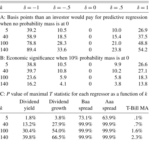
Table 6 compares the economic significance of the predictive regression with the statistical significance of the regressors. The economic significance of the regression is reported in panels A and B of Table 6 by showing the amount that an investor would be willing to pay, in basis points, for the information that the conditional mean liesδregression standard deviations from the unconditional mean. Panel A shows the value ofXT askvaries for an investor that entertains no uncertainty about the model of predictability in his or her prior, whereas panel B reports the value for an investor that averages over the 2k models. To quantify the statistical significance of the regressors, panel C of Table 6 presents thetstatistics andpvalues associated with the maximal tstatistic for each of the original five predictive variables. Thesepvalues are calculated as the probability un-der the null hypothesis of getting a t statistic at least this ex-treme given that the investor samples a total ofkdifferent vari-ables.
Comparing panels A and C, it is evident that the value of the predictive regression to an investor who knows the model of predictability has no relationship with the variables’ statis-tical significance. Whereas thep value on all of thetstatistics decrease when 135 simulated variables are added to the regres-sion, the investor increases from 39.2 to 89.4 the basis points she would pay to know that the conditional mean is one re-gression standard deviation below the unconditional mean. The same is not true, however, for the investor in panel B that av-erages over the 2kmodels. This investor would pay 38.8 basis points for the information that the conditional mean of the re-gression was one standard deviation below its mean when there
Table 6. Economic and statistical significance of the regression when R2increases as variables are added
k δ= −1 δ= −.5 δ=0 δ=.5 δ=1
A: Basis points than an investor would pay for predictive regression when no probability mass is at 0
5 39.2 10.5 0 10.0 26.9
40 58.9 18.5 0 15.4 37.5
100 78.8 28.3 0 21.0 48.8
140 89.4 33.6 0 23.8 54.2
B: Economic significance when 10% probability mass is at 0
5 38.8 10.5 0 9.9 26.6
40 39.7 10.8 0 10.2 27.1
100 23.6 5.9 0 5.8 18.3
140 16.2 4.1 0 3.8 13.8
C:Pvalue of maximalTstatistic for each regressor as a function ofk
Dividend Dividend Baa Aaa
k yield growth spread spread T-Bill MA
5 1.8% 3.8% 73.1% 63.9% .1%
40 13.2% 27.9% 99.9% 99.9% .7%
100 30.4% 54.0% 99.9% 99.9% 1.6%
140 39.8% 66.5% 99.9% 99.9% 2.3%
NOTE: This table reports the statistical and economic significance of the regressors. Pan-els A and B report the number of basis points that an investor would be willing to give up to obtainXT, the vector containing the values of thekpredictive variables at timeT, to
construct the predictive density of future returns,p(rT+1|T). The value of the
informa-tion to the investor is listed as a funcinforma-tion ofk, the number of variables, andδ, the number of regression standard deviations that the regression forecast is above or below the uncon-ditional mean. In panel A the investor places no point mass at 0, whereas in panel B the investor places 10% probability that returns are iid and then averages over the 2kmodels.
Panel C reports thepvalue associated with getting atstatistic at least as extreme as the one reported in the original predictive regression given that the variable was chosen from amongkvariables.
are 5 regressors in the model, but only 16 basis points when there are 140. Once again, parsimony is only rewarded by the investor that averages over the predictive models. Compare this with the statistical significance reported in panel C. Notice that askincreases from 5 to 140, only 1 of the original 5 variables maintains statistical significance. That one variable, the T-Bill minus its 1-year moving average, has atstatistic of−3.8. Even if that regressor had been chosen randomly from among 140 variables, it would be significant at the 2.25% level in a two-tailed test. Compare this to the other 4 variables whosepvalues are all>.10 once 35 additional regressors have been added to the analysis. Thus the investor in panel B ascribes value to the predictive regression, because the data support the hypothesis that at least this one variable is capable of predicting returns.
To illustrate that the value of the regression’s information is due to the presence of this one statistically significant variable, Table 7 repeats the analysis of panel B when the T-Bill minus its 1-year moving average variable is removed from the regres-sion. Excluding this variable drops the value of the predictive regression from 16 basis points to only 3 when 135 variables are added to the original regression. This implies that the eco-nomic significance of the predictive regression is driven by the presence of the one statistically significant variable as measured by the maximal tstatistic, the T-Bill minus its 1-year moving average. Once again, the economic significance tends to follow the statistical significance when model uncertainty is treated in a similar fashion across the two metrics.
Table 7. Economic significance of the regression when the T Bill minus its moving average is removed
k δ= −1 δ= −.5 δ=0 δ=.5 δ=1
4 20.7 5.2 0 5.1 16.8
39 8.5 2.1 0 2.1 8.2
99 6.9 1.7 0 1.7 6.8
139 3.2 .8 0 .8 3.1
NOTE: This table repeats the analysis of panel B of Table 6 while excluding one pre-dictive regressor, the 1-month T-Bill minus its 1-year moving average. The value of the information to the investor is listed as a function ofk, the number of variables, andδ, the number of regression standard deviations that the regression forecast is above or below the unconditional mean.
5. CONCLUSIONS
The discrepancy between the economic and statistical met-rics reported by Kandel and Stambaugh (1996) is largely at-tributable to the treatment of the investor’s prior. KS repre-sented the investor’s uncertainty about the predictive regression by centering the prior over the slope parameters at 0. The more informative the prior, the more probability mass close to 0, and the more skeptical the investor about the predictive relationship. Nevertheless, because there is no point mass at 0 in the prior to represent the possibility that returns are not predictable, all of the probability mass in the posterior must lie under the model of predictability. Such a prior violates Cromwell’s rule: Never place probability one on any model. This prior specification makes it impossible for the investor to use the data to analyze the relative strength of the point-null hypothesis that returns are not predictable in relation to the alternative hypothesis that re-turns are predictable.
Placing point mass in the investor’s prior that the regression slope coefficients are 0 does away with the tension between the economic and statistical metrics by allowing the investor to in-clude the cost of type I errors in his or her decision. The end re-sult is that the posterior probability on the point-null hypothesis (i.e., returns are not predictable) shrinks the conditional mean from the predictive regression toward the unconditional mean and tempers the investor’s portfolio reallocation. This shrink-age greatly reduces the portfolio reallocation because, as shown in equation (4), the predictive conditional mean is a function of the asset’s volatility. As Jorion (1991) noted, variances are much larger than means in these portfolio allocation problems. Thus small perturbations in the regressors lead to large percent-age changes in the regression’s conditional mean. Indeed, the more volatile the asset, the larger the change in the regression’s conditional mean. As a result, Kandel and Stambaugh (1996) observed large portfolio reallocations, because their investor only uses the conditional predictive mean in forecasting next month’s return. Tempering these shifts in the conditional mean through the use of a point-null hypothesis, as we do in this arti-cle, is akin to the shrinkage literature of Merton (1980), Jorion (1986), and Frost and Savarino (1986), where the expected re-turns on multiple risky portfolios are estimated jointly.
Nevertheless, the question of the predictability of asset re-turns remains an unanswered question in the economic met-ric. Whereas the KS prior is not appropriate for analyzing the question of asset return predictability, it is not clear what prior is. In this article we have opted to use a point-null hypothe-sis to simply illustrate the importance of Cromwell’s rule by
Roskelley: Role of Prior in Portfolio Allocation Problem 235
introducing type I errors into the investor’s portfolio alloca-tion problem. Poirier (1988), however, argued that the use of a point-null hypothesis lacks economic meaning and is awkward at best in a Bayesian framework. Robert (2001) pointed out that an interval-null hypothesis could be used instead of a single point. For instance, in this asset allocation problem, the prob-ability mass around 0 could be expanded to preclude trading when transaction costs outweigh the perceived benefits. Such a prior would tip the results further in favor of rejecting the model of predictability.
But Jeffreys and Neyman likely would argue that hypothesis testing should be conducted between two well-defined compet-ing models when possible (see Berger 2003). Although asset return predictability is one instance in which academic interest lies in measuring the evidence in favor of a point-null hypothe-sis (i.e., returns are not predictable), including structural uncer-tainty into the predictive model would seem to be a logical next step. Although allowing the investor to average over predic-tive linear models is a move in that direction, the analysis also could be expanded to include nonlinear structural models. This would more accurately represent an investor’s uncertainty about the structural form of the predictive model. Although Bayesian model averaging could then be used to form the composite pre-dictive density for returns using a combination of linear and nonlinear predictive models, Cromwell’s rule would still apply: Never discount the possibility that the correct model has not been included. Perhaps, then, the inclusion of an unspecified alternative hypothesis, similar to robust control theory, could prove useful. Although Hansen and Sargent (2005) provided a useful overview of implementing modern control theory into economic problems, little work has been done in this area in finance.
One other possible consideration in measuring the economic significance of predictability is the choice of the utility, or loss, function. The fact that portfolio allocations are so sensitive to the estimated means might indicate that using a power utility function is misleading. For instance, the equity premium puz-zle literature started by Mehra and Prescott (1985) shows that historical risk premia imply risk aversion levels that are not con-sistent with observed investor portfolio holdings. Benartzi and Thaler (1995), among others, have attempted to attribute this to misspecification of the investor’s utility function. In any case, more thought should go into the choice of both the investor’s prior and the investor’s underlying loss function before the eco-nomic metric can be meaningfully interpreted.
ACKNOWLEDGMENTS
The author thanks Christopher Lamoureux, Hilde Patron, Lu-bos Pastor, Darrel Duffie, an anonymous referee, and the sem-inar participants of the University of Arizona and Brigham Young University for their comments and feedback.
APPENDIX: CONSTRUCTION OF POSTERIOR DENSITIES
Looking more closely at the derivation of the posterior
p(rT+1|T), we follow in part the exposition of Koop (2003) and Madigan and York (1995). To get the predictive density of
modelMifor the monthly returnrT+1, we combine the
poste-rior density on the parameters with the predictive likelihood to get the joint density for the parameters and future returns,
p(rT+1, βi, σi|T,Mi)
=p(βi, σi|T,Mi)·p(rT+1|βi, σi,XT,Mi). Integrating over the unknown parametersβandσ and then tak-ing a probability-weighted average over the 2kmodels defined by thekvariables gives the predictive density forrT+1, the
con-ditional return for the upcoming month,
p(rT+1|T)=
2k
i=1
p(Mi) p(rT+1, βi, σi|T,Mi)dβidσi .
Due to the use of conjugate priors as specified in Section 3.2, the posterior distribution ofβ andσ is known for each model (see Zellner 1971; Koop 2003). But the composite posterior dis-tribution of the parameters is not a known density, because we must average over the 2k candidate models. To take the draws from p(rT+1|T), first draws from the parameters and draws from the predictive likelihood must be made. Draws from the posterior on the parameters are made using the Markov chain Monte Carlo model composition (MC3) technique developed by Madigan and York (1995). A candidate model,M∗, is drawn randomly and with equal probability from the set of models that includes the current model Mi and all models that delete one regressor,Mi−1, as well as all models that add one regres-sor,Mi+1. Once the candidate modelM∗has been selected, the probability of accepting the candidate model is calculated as
α(Mi,M∗)=min
p(r|M∗)p(M∗)
p(r|Mi)p(Mi)
,1
,
where p(r|M∗) andp(r|Mi) are the marginal distributions of the observed data given the model and p(M∗) andp(Mi) are
the prior probabilities on the models. Once the probability
α(Mi,M∗)has been calculated, a draw from a uniform (0,1) distribution is made; if the draw is less than α(Mi,M∗), then the candidate model is accepted, and the new draw from the parameters comes from the model M∗. If the draw is less
thanα(Mi,M∗), then the parameters are drawn from the cur-rent model, Mi. The procedure continues until convergence is achieved. In this case it is important that convergence is ana-lyzed using the predictive distribution of returns from the con-ditional mean usingXT, not the unconditional mean obtained using the average of the regressors. Although all models have the same unconditional mean, they each have different condi-tional means depending on XT, making maximization of the expected utility function difficult and computationally costly as
kincreases. Geweke (1994), for instance, noted that computa-tional time is “roughly proporcomputa-tional to the cube of the number of regressors.” Convergence is checked using the convergence diagnostics of Geweke (1992) and Raftery and Lewis (1992).
Once the draws on the parameters have been made and an-alyzed for convergence, the predictive density may then be formed for use in the investor’s expected utility maximization problem. The predictive density for returns is constructed by adding in the predictive likelihood to the posterior density of the
parameters and integrating over the parameter space as in equa-tion (3). This is done by calculating the expected return condi-tional on the vector of predictive variables,XT, for each draw onβ from the posterior distribution. Each conditional return is then added to a normally distributed error term,ǫt∼N(0, σ2), as in equation (1). To integrate over the error term we combine each of the draws on the parameters with 5,000 draws on the er-ror term. Thus if there areidraws on the parameters, then there will be 5,000ireturns forming the posterior predictive distrib-ution for the 1-month-ahead continuously compounded return. The 5,000idraws from the predictive density are then used to perform the integration in equation (2), giving the expected util-ity as a function of the portfolio weights. Maximization of the utility function is carried out using a simple quadratic interpo-lation method.
[Received December 2005. Revised November 2006.]
REFERENCES
Avramov, D. (2002), “Stock Return Predictability and Model Uncertainty,”
Journal of Financial Economics, 64, 423–458.
Benartzi, S., and Thaler, R. H. (1995), “Myopic Loss Aversion and the Equity Premium Puzzle,” Quarterly Journal of Economics, 110, 73–92.
Berger, J. O. (2003), “Could Fisher, Jeffreys and Neyman Have Agreed on Test-ing?”Statistical Science, 18, 1–32.
Brennan, M., and Xia, Y. (2001), “Asset Pricing Anomalies,”Review of Finan-cial Studies, 14, 905–942.
Campbell, J., and Yogo, M. (2005), “Efficient Tests of Stock Return Predictabil-ity,”Journal of Financial Economics, 81, 27–60.
Chen, M., Shao, Q., and Ibrahim, J. G. (2000), Monte Carlo Methods in Bayesian Computation, New York: Springer-Verlag.
Clyde, M., and George, E. I. (2004), “Model Uncertainty,”Statistical Science, 19, 81–94.
Cremers, M. (2002), “Stock Return Predictability: A Bayesian Model Selection Perspective,”Review of Financial Studies, 15, 1223–1249.
Ferson, W., Sarkissian, S., and Simin, T. (2003), “Spurious Regressions in Fi-nancial Economics?”Journal of Finance, 58, 1393–1413.
Foster, F., Smith, T., and Whaley, R. (1997), “Assessing Goodness of Fit of Asset Pricing Models: The Distribution of the MaximalR2,”Journal of Fi-nance, 52, 591–607.
Frost, P. A., and Savarino, J. E. (1986), “An Empirical Bayes Approach to Ef-ficient Portfolio Selection,”Journal of Financial and Quantitative Analysis, 21, 293–305.
Geweke, J. (1992), “Evaluating the Accuracy of Sampling-Based Approaches to Calculating Posterior Moments,” inBayesian Statistics 4, eds J. Bernardo, J. Berger, A. Dawid, and A. Smith, Oxford, U.K.: Clarendon Press, pp. 169–193.
(1994), “Variable Selection and Model Comparison in Regression,” in
Bayesian Statistics 5, eds. J. Bernardo, J. Berger, A. Dawid, and A. Smith, Oxford, U.K.: Oxford University Press, pp. 609–620.
Hansen, L. P., and Sargent, T. J. (2005), “Robustness,” working monograph, University of Chicago, Dept. of Economics.
Ibbotson Associates (1997), Stocks, Bonds, Bills, and Inflation Yearbook, Chicago: Author.
Jorion, P. (1986), “Bayes–Stein Estimation for Portfolio Analysis,”Journal of Financial and Quantitative Analysis, 21, 279–292.
(1991), “Bayesian and CAPM Estimators of the Means: Implications for Portfolio Selection,”Journal of Banking and Finance, 15, 717–727. Kandel, S., and Stambaugh, R. (1996), “On the Predictability of Stock Returns:
An Asset Allocation Perspective,”Journal of Finance, 51, 385–424. Koop, G. (2003),Bayesian Econometrics, West Sussex, U.K.: Wiley. Lamoureux, C. G., and Zhou, G. (1996), “Temporary Components of Stock
Returns: What Do the Data Tell Us?” Review of Financial Studies, 9, 1033–1059.
Lindley, D. (1957), “A Statistical Paradox,”Biometrica, 44, 187–192. Madigan, D., and York, J. (1995), “Bayesian Graphical Models for Discrete
Data,”International Statistical Review, 63, 215–232.
Mehra, R., and Prescott, E. C. (1985), “The Equity Premium: A Puzzle,” Jour-nal of Monetary Economics, 15, 145–161.
Merton, R. C. (1980), “On Estimating the Expected Return on the Market: An Exploratory Investigation,”Journal of Financial Economics, 8, 323–361. Pastor, L. (2000), “Portfolio Selection and Asset Pricing Models,”Journal of
Finance, 55, 179–223.
Pastor, L., and Stambaugh, R. (2000), “Comparing Asset Pricing Models: An Investment Perspective,”Journal of Financial Economics, 56, 335–381. Poirier, D. J. (1988), “Frequentist and Subjectivist Perspectives on the
Prob-lems of Model Building in Economics,”Journal of Economic Perspectives, 2, 121–144.
Raftery, A. E., and Lewis, S. M. (1992), “One Long Run With Diagnostics: Im-plementation Strategies for Markov Chain Monte Carlo,”Statistical Science, 7, 493–497.
Richardson, M. (1993), “Temporary Components of Stock Prices: A Skeptic’s View,”Journal of Business & Economic Statistics, 11, 199–207.
Robert, C. P. (2001),The Bayesian Choice, New York: Springer-Verlag. Stambaugh, R. (1999), “Predictive Regressions,”Journal of Financial
Eco-nomics, 54, 375–421.
Sullivan, R., Timmermann, A., and White, H. (2001), “Dangers of Data-Driven Inference: The Case of Calendar Effects in Stock Returns,”Journal of Econo-metrics, 105, 249–286.
Torous, W., Valkanov, R., and Yan, S. (2004), “On Predicting Stock Returns With Nearly Integrated Explanatory Variables,”Journal of Business, 77, 937–966.
Tu, J., and Zhou, G. (2004), “Data-Generating Process Uncertainty: What Dif-ference Does It Make in Portfolio Decisions?”Journal of Financial Eco-nomics, 72, 385–421.
White, H. (2000), “A Reality Check for Data Snooping,”Econometrica, 68, 1097–1126.
Zellner, A. (1971),An Introduction to Bayesian Inference in Econometrics, New York: Wiley.
(1986), “On Assessing Prior Distributions and Bayesian Regression Analysis Withg-Prior Distributions,” inBayesian Inference and Decision Techniques: Essays in Honor of Bruno de Finetti, eds. P. K. Goel and A. Zell-ner, Amsterdam: North-Holland, pp. 233–243.