A Kinematic Analysis and Evaluation of Planar Robots
Designed From Optimally Fault-Tolerant Jacobians
Khaled M. Ben-Gharbia, Student Member, IEEE,
Anthony A. Maciejewski, Fellow, IEEE,
and Rodney G. Roberts, Senior Member, IEEE
Abstract—It is common practice to design a robot’s kinematics from the desired properties that are locally specified by a manipulator Jacobian. In this work, the desired property is fault tolerance, defined as the post-failure Jacobian possessing the largest possible minimum singular value over all possible locked-joint failures. A mathematical analysis based on the Gram matrix that describes the number of possible planar robot designs for optimally fault-tolerant Jacobians is presented. It is shown that rearranging the columns of the Jacobian or multiplying one or more of the columns of the Jacobian by±1 will not affect local fault tolerance; however, this will typically result in a very different manipulator. Two examples, one that is optimal to a single joint failure and the second that is optimal to two joint failures, are analyzed. This analysis shows that there is a large variability in the global kinematic properties of these designs, despite being generated from the same Jacobian. It is especially surprising that major differences in global behavior occurs for manipulators that are identical in the working area.
Index Terms—Fault-tolerant robots, robot kinematics, redundant
robots.
I. I
NTRODUCTIONThe design and operation of fault-tolerant manipulators is critical
for applications in remote and/or hazardous environments where
rou-tine maintenance and repair are not possible. The failure rates for
components in such harsh environments are relatively high [1]–[3].
1Example applications include space exploration [5], [6], underwater
exploration [7], and nuclear waste remediation [8], [9], where there has
been a great deal of research to improve manipulator reliability [3], [10],
design fault-tolerant robots [11], [12], and determine mechanisms for
analyzing [13], detecting [14], [15], identifying [16]–[18], and
recov-ering [19]–[22] from failures. Many of these component failures will
result in a robot’s joint becoming immobilized, i.e., a locked joint
fail-ure mode [14], [23]. In addition, component failfail-ures that result in other
common failure modes, e.g., free-swinging joint failures [24], [25], are
frequently transformed into the locked joint failure mode by failure
recovery mechanisms that employ fail safe brakes [26].
A large body of work on fault-tolerant manipulators has focused on
the properties of kinematically redundant robots, both in serial or
par-allel form [27]–[31]. These analyses have been performed both on the
Manuscript received July 7, 2013; accepted November 4, 2013. Date of pub-lication January 27, 2014; date of current version April 1, 2014. This paper was recommended for publication by Associate Editor J. Peters and Editor C. Torras upon evaluation of the reviewers’ comments. This work was supported in part by the National Science Foundation under Contract IIS-0812437.
K. M. Ben-Gharbia and A. A. Maciejewski are with the Department of Electrical and Computer Engineering, Colorado State University, Fort Collins, CO 80523-1373, USA (e-mail: [email protected]; [email protected]).
R. G. Roberts is with the Department of Electrical and Computer Engineer-ing, Florida A&M–Florida State University, Tallahassee, FL 32310-6046, USA (e-mail: [email protected]).
Color versions of one or more of the figures in this paper are available online at http://ieeexplore.ieee.org.
Digital Object Identifier 10.1109/TRO.2013.2291615
1One recent example is the Fukushima nuclear reactor accident, where robot
component failures were not only likely, but inevitable [4].
local properties associated with the manipulator Jacobian [32]–[35]
as well as the global characteristics such as the resulting workspace
following a particular failure [36]–[39]. (Clearly both local and global
kinematic properties are related, e.g., workspace boundaries correspond
to singularities in the Jacobian.) In this work it is assumed that one is
given a set of local performance constraints that require a manipulator
to function in a configuration that is optimal under normal operation and
after an arbitrary single joint fails and is locked in position. Specifically,
the desired Jacobian matrix must be isotropic, i.e., it should possess all
equal singular values prior to a failure, and have equal minimum
sin-gular values for every possible single column being removed. Because
these constraints do not result in a unique manipulator, one can then
use global characteristics to distinguish between multiple manipulators
that meet the local design criteria.
In this work, we focus on the characteristics of planar manipulator
designs. This does not necessarily mean that the physical robot must
operate in only two dimensions. For example, many robot designs can
be decomposed into a planar portion along with an orthogonal portion,
e.g., SCARA robots. Thus one approach to obtaining a higher reliability
robot with a simpler design is to only apply the fault-tolerant techniques
discussed here to the planar component.
The remainder of this paper is organized in the following manner.
A local definition of failure tolerance centered on desirable properties
of the manipulator Jacobian is mathematically defined in the next
sec-tion. In Section III, the Gram matrix is used to describe all Jacobians
with the same optimal fault tolerance properties. These results are used
to present illustrative examples of manipulator designs that are
gener-ated from optimally fault-tolerant Jacobians in Section IV. The global
properties of manipulators that possess the same Jacobian are analyzed
and compared in Section V. An example is shown of an optimally
fault-tolerant eight degree-of-freedom manipulator operating in a fully
six-dimensional task space is shown in Section VI. The conclusions of
this work are then presented in Section VII.
II. B
ACKGROUND ONO
PTIMALLYF
AULT-T
OLERANTJ
ACOBIANSAs was done in [40], the dexterity of a manipulator is quantified in
terms of the properties of the manipulator Jacobian matrix that relates
end-effector velocities to joint angle velocities. The Jacobian will be
denoted by the
m
×
n
matrix
J
, where
m
is the dimension of the task
space and
n
is the number of degrees-of-freedom of the manipulator.
For redundant manipulators
n > m
, and the quantity
n
−
m
is the
degree of redundancy. The manipulator Jacobian can be written as a
collection of columns
J
m×n= [
j
1j
2· · ·
j
n]
(1)
where
j
irepresents the end-effector velocity due to the velocity of joint
i
. For an arbitrary single joint failure at joint
f
, assuming that the failed
joint can be locked, the resulting
m
by
n
−
1
Jacobian will be missing
the
f
th column, where
f
can range from 1 to
n
. This Jacobian will be
denoted by a preceding superscript so that in general
f
J
m×(n−1 )
= [
j
1j
2. . . j
f−1j
f+ 1. . . j
n]
.
(2)
The properties of a manipulator Jacobian are frequently quantified in
terms of the singular values, denoted
σ
i, which are typically ordered so
that
σ
1≥
σ
2≥ · · · ≥
σ
m≥
0
. Most local dexterity measures can be
defined in terms of simple combinations of these singular values such
as their product (determinant) [41], sum (trace), or ratio (condition
number) [42]–[44]. The most significant of the singular values is
σ
m,
the minimum singular value, because it is by definition the measure
of proximity to a singularity and tends to dominate the behavior of
both the manipulability (determinant) and the condition number. The
minimum singular value is also a measure of the worst-case dexterity
over all possible end-effector motions.
The definition of failure tolerance used in this work is based on the
worst-case dexterity following an arbitrary locked joint failure. Because
fσ
m
denotes the minimum singular value of
fJ,
fσ
mis a measure of
the worst-case dexterity if joint
f
fails. If all joints are equally likely
to fail, then a measure of the worst-case failure tolerance is given by
K
=
min
nf= 1
(
f
σ
m
)
.
(3)
Physically, this corresponds to minimizing the worst-case increase in
joint velocity when a joint is locked and the others must accelerate to
maintain the desired end effector trajectory. In addition, maximizing
K
is equivalent to locally maximizing the distance to the postfailure
workspace boundaries [1]. To insure that manipulator performance
is optimal prior to a failure, an optimally failure tolerant Jacobian
is further defined as having all equal singular values because of the
desirable properties of isotropic manipulator configurations [42]–[44].
Under these conditions, to guarantee that the minimum
fσ
m
is as large
as possible, they should all be equal. It is easy to show [33] that the
worst-case dexterity of an isotropic manipulator that experiences a
single joint failure is governed by the inequality
n
where
σ
denotes the norm of the original Jacobian. The best case of
equality occurs if the manipulator is in an optimally failure tolerant
configuration. The above inequality makes sense from a physical point
of view because it represents the ratio of the degree of redundancy to
the original number of degrees of freedom.
Using the above definition of an optimally failure tolerant
configu-ration, one can identify the structure of the Jacobian required to obtain
this property [45].
2In particular, one can show that the optimally
fail-ure tolerant criteria requires that each joint contributes equally to the
null space of the Jacobian transformation [34]. Physically, this means
that the redundancy of the robot is uniformly distributed among all
the joints so that a failure at any joint can be compensated for by the
remaining joints. Therefore, in this work, an optimally failure tolerant
Jacobian is defined as being isotropic, i.e.,
σ
i=
σ
for all
i
, and
hav-ing a maximum worst-case dexterity followhav-ing a failure, i.e., one for
which
fσ
m=
σ
n−m
n
for all
f
. The second condition is equivalent
to having the columns of the Jacobian have equal norms.
The simplest example of an optimally failure tolerant configuration
is given by the following Jacobian for a three degree-of-freedom planar
manipulator:
illustrates that each joint contributes equally to the null space motion,
thus distributing the redundancy proportionally to all degrees of
free-dom. Geometrically, it is easy to see that the three vectors
j
1, j
2, and
j
3are all
120
◦apart, which results in a balanced coverage of the planar
2Note that our approach does not depend on our choice of fault tolerance
measure. Any fault-tolerant measure, e.g., relative manipulability, can be used to define a locally optimally failure tolerant Jacobian. In fact, any local desired property defined by a Jacobian can be used in our approach.
workspace. If the three possible joint failures are considered, one can
show that
for
f
= 1
to
3
, which satisfies the optimally failure tolerant criterion.
Given this example of an optimally failure tolerant
J
, one might be
interested in designing the kinematics for a manipulator that would
possess these qualities. In the next section, the Gram matrix is used to
analyze the different number of manipulator kinematics that can result
from a given fault-tolerant Jacobian.
III. F
AULTT
OLERANCE AND THEG
RAMM
ATRIXAs first shown in [40], the Gram matrix
G
=
J
TJ
(7)
provides insight into the geometry and fault tolerance of a manipulator
design. Here, the Jacobian
J
can be the positional, orientational, or the
manipulator Jacobian. Some care concerning units should be exercised
in the case of the manipulator Jacobian or when there is a mixture of
revolute and prismatic joints. When a Jacobian is isotropic, the Gram
matrix takes on a particularly simple form: If the singular values of
J
are equal to 1, then
G
=
J
TJ
=
I
−
N N
T, where the
n
×
(
n
−
m
)
matrix
N
consists of
(
n
−
m
)
orthonormal null vectors of
J
. In the case
of a manipulator with a single degree of redundancy,
G
=
I
−
n
ˆ
Jn
ˆ
TJ,
where
n
ˆ
Jis the unit length null vector when
J
is in a non-singular
configuration. The requirement for optimal fault tolerance specifies
further conditions on the null space matrix
N
. Specifically, the rows of
N
must all have the same norm
n−nmand be spread out in a sense
that will be made precise later.
Once an optimal Gram matrix is determined, an obvious and
im-portant question is to characterize all the corresponding Jacobians and
Denavit and Hartenberg (DH) parameters for the corresponding
manip-ulators. Clearly, a simple change in the base frame orientation through
rotation and/or reflection will not change the basic robot structure. The
difference in this case is simply a pre-multiplication of the Jacobian
by an orthogonal matrix. For the sake of discussion, we will say that
two configurations are
equivalent
if their corresponding Jacobians
dif-fer only by a pre-multiplication by an orthogonal matrix
Q
. For any
n
degree-of-freedom revolute jointed planar manipulator, denoted by
n
-R, it can be shown that two full rank Jacobians
J
and
J
′are
equiv-alent if and only if
(
J
′)
TJ
′=
J
TJ
, i.e., if their Gram matrices are
equal.
Two planar
n
-R manipulators with equivalent Jacobians have
essen-tially the same DH parameters, so the corresponding robot
configura-tions can be considered to be the same in that sense. This is because
when there is a change in the orientation of the base frame, either
through a rotation or a combination of a rotation and reflection, the
new Jacobian merely differs from the original by a multiplication by an
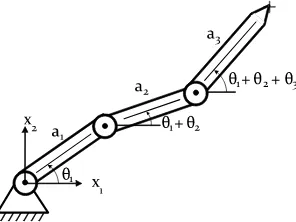
orthogonal matrix. This is nicely illustrated for a planar 3R manipulator
(see Fig. 1) that has a Jacobian of the form
J
(
θ
1, θ
2, θ
3) =
where the fixed
a
i’s are the link lengths, the variable
θ
i’s are the joint
angles, and the remaining DH parameters have values equal to zero.
(The notation
s
i j kand
c
i j kindicates
sin(
θ
i+
θ
j+
θ
k)
and
cos(
θ
i+
Fig. 1. A simple three degree-of-freedom planar manipulator.
to isolate specific terms in (8). If the base frame is changed by a rotation,
represented here by a
2
×
2
rotation matrix
R
(
φ
)
, the manipulator’s
Jacobian becomes
J
′(
θ
1
, θ
2, θ
3) =
R
(
φ
)
J
(
θ
1, θ
2, θ
3) =
J
(
θ
1+
φ, θ
2, θ
3)
(9)
where
R
(
φ
)
is the standard rotation matrix corresponding to a
counter-clockwise rotation of
φ
radians about the
x
3-axis. The DH parameters
of the robot corresponding to the new Jacobian
J
′(
θ
1
, θ
2, θ
3)
are the
same as they were for
J
with the exception that
θ
1is now replaced with
θ
1+
φ
. Consider now the reflection matrix
F
= diag(
−
1
,
1)
, which
corresponds to a reflection about the
x
2–
x
3plane. Then, the modified
Jacobian resulting from pre-multiplying by
F
is
J
′(
θ
1, θ
2, θ
3) =
F J
(
θ
1, θ
2, θ
3) =
J
(
−
θ
1,
−
θ
2,
−
θ
3)
.
(10)
The new DH parameters are the same except that the joint angles are
the negatives of the original joint angles, giving a left-handed version of
the same robot. More generally, any orthogonal matrix can be written
in the form
R
(
φ
)
or
Q
=
R
(
φ
)
F
for a suitable angle
φ
so that
pre-multiplying (1) by Q results in the Jacobian
QJ
(
θ
1, θ
2, θ
3) =
J
(
−
θ
1+
φ,
−
θ
2,
−
θ
3)
.
(11)
Because optimal fault tolerance can be formulated in terms of the
Gram matrix, it is desirable to identify the family of DH parameter sets
that result in optimally fault-tolerant configurations. The unique DH
parameters for a planar 3R robot are easily obtained from (8) by
exam-ining the matrix
[
j
1−
j
2j
2−
j
3j
3]
, e.g., the column norms of this
new matrix are equal to the corresponding
a
ivalues. This observation
generalizes for any planar
n
-R robot. One could also obtain the values
for
a
ifrom the Gram matrix by noting that for
i
= 1
,
2
, . . . , n
−
1
manipulators, a given Gram matrix
G
determines a family of equivalent
manipulators, each with the same set of
a
iparameters determined by
the square root of a simple linear combination of elements in
G
.
Another important question is whether one can identify other
opti-mally fault-tolerant designs from a given Jacobian that are not
equiv-alent by pre-multiplication by an orthogonal matrix. It is clear from
the definition of optimal fault tolerance that rearranging the columns
of
J
or multiplying one or more of the columns of
J
by
−
1
will not
affect local fault tolerance; however, this will typically result in a very
different manipulator. We will say that
J
and
J
′are
similar
if one is
ob-tained from the other by permuting and/or multiplying the columns of a
Jacobian by
−
1
. In other words,
J
and
J
′are similar if
J
′=
J S
, where
S
is an
n
×
n
matrix corresponding to the desired signed permutation
of the columns of
J
. For convenience, we will say that
J
and
J
′are
nontrivially similar
if
S
=
±
I
. We are interested in similar Jacobians
because they share the same fault tolerance properties but generally
correspond to fundamentally different manipulators. The Gram matrix
G
′corresponding to
J
′is obtained from the original Gram matrix
G
simply by applying the same row and column operations that were
used to obtain
J
′from
J
. Consequently, one can easily obtain the
a
i
parameters for any similar Jacobian directly from the original
G
for
the case of planar revolute manipulators. This will be illustrated in the
next section.
IV. E
XAMPLES OFM
ANIPULATORS WITHO
PTIMALF
AULT-T
OLERANTJ
ACOBIANSAs mentioned earlier [40], the restrictions imposed by this definition
of fault tolerance limits the number of possible robot geometries. To
see this, consider the problem of identifying all planar 3R manipulators
with an optimally fault-tolerant Jacobian
J
. When the
2
×
3
Jacobian
J
is isotropic with unit singular values, we have
G
=
J
TJ
=
I
−
n
ˆ
Jn
ˆ
TJ.
(14)
Fault tolerance requires that the components of
n
ˆ
Jhave the same
magnitude. However, replacing
ˆ
n
Jwith
−
n
ˆ
Jdoes not affect (2), so
we only need to check the four cases
ˆ
n
J= 1
/
√
3 [1
±
1
±
1]
T.
These four unit null vectors determine four families of nonequivalent
Jacobians, each corresponding to one of the four possibilities for
I
−
ˆ
n
Jn
ˆ
TJ, which together identify all Jacobians that are optimally fault
tolerant.
The optimally fault-tolerant Jacobian given in (5) corresponds to the
case when the elements of
n
ˆ
Jare all positive and equal. In this case,
the Gram matrix corresponding to the positional Jacobian is
G
=
The link length parameters for this particular
G
are then
a
1=
a
2=
Gram matrices obtained through permutations and multiplications by
−
1
as described earlier, one can easily deduce that the only possible link
length values for an optimally fault-tolerant planar 3R manipulator are
L
l=
√
2
and
L
s=
2
/
3
, which are obtained by using off-diagonal
elements that equal
±
13
and diagonal elements equal to
23
. Furthermore,
the square root of a diagonal value of
G
is equal to the distance of the
end effector from the corresponding joint. In this case, each joint lies
on a circle of radius
2
/
3
centered at the end effector with the two
possible link lengths
√
2
and
2
/
3
, which necessarily place the joints
on the vertices of an inscribed hexagon. The four optimally
fault-tolerant manipulators are described by the link lengths in Table I and
illustrated in Fig. 2.
TABLE I
FOURDIFFERENTLINKLENGTHCOMBINATIONS OF(5)
(c) (d)
(a) (b)
Fig. 2. A simple three degree-of-freedom planar robot that corresponds to the optimal fault-tolerant Jacobian given by (5) is shown in (d). The three other manipulators that have the same properties of the Jacobian in (5) are shown in (a)–(c).
successive rows are
45
◦. Any other null space matrix related to
N
by a
row permutation and/or the multiplication of one or more rows by
−
1
will also result in an optimally fault-tolerant Jacobian. The
correspond-ing Jacobian would be given by applycorrespond-ing the same operations to the
columns of the original Jacobian. An example of a suitable Jacobian is
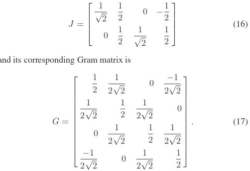
J
=
and its corresponding Gram matrix is
G
=
From the diagonal elements of (17), it follows that the joints
of the manipulator are located on a circle of radius
1
/
√
2
cen-tered at the end effector. The link lengths for this particular
G
are
a
i=
low that the four potential link lengths for similar Gram matrices
are
L
a=
quently, it follows that the joints of an optimally fault-tolerant planar
4R manipulator appear on the vertices of an octagon inscribed on a
TABLE II
FOURTEENDIFFERENTLINKLENGTHCOMBINATIONS OF(16)
circle of radius
√12
centered at the end effector. The list of all possible
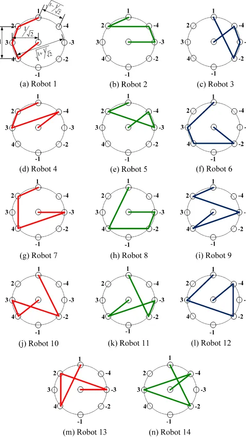
manipulators is presented in Table II and depicted in Fig. 3.
These possible robots resulted from the fact that all possible
permu-tations and multiplications by
−
1 of the columns of (16) result in the
second diagonal of (17) (i.e., the diagonal above the main diagonal)
being in exactly one of three forms, i.e., (
x
,
y
,
z
), (
x
,0,
z
), or (0,
y
,0),
where each
x, y
, and
z
can be either
±
12√2
. Thus, the total number of
distinct link lengths is:
2
3= 8
for the (
x
,
y
,
z
) case plus
2
2= 4
for the
(
x
,0,
z
) case plus
2
1= 2
for the (0,
y
,0) case resulting in 14 different
manipulator designs. Note that not every manipulator with the property
that it’s joints are located in the vertices of this octagon are optimally
fault tolerant, but the Gram matrix clearly identifies this requirement
for the family of optimally fault-tolerant manipulators.
The next section discusses the global fault-tolerant behavior of both
the 3R and 4R families of manipulators, and shows how the robots
within the same family are still quite different as they act differently
beyond the design point.
V. A
NALYSIS ANDC
OMPARISON OFM
ANIPULATORD
ESIGNSThe fact that there are multiple manipulator designs with the same
desired local fault tolerance properties allows one to use other criteria
to select a preferred design. In particular, while the robots all share the
same local properties at the given configuration, they are quite different
in terms of their global properties. For example, first consider the 3R
robots defined in Table I and Fig. 2. Even when joint limits are not
considered, their workspaces are quite different, e.g., the maximum
reach will be either
3
L
s,
2
L
s+
L
l, or
L
s+ 2
L
l. More importantly,
if one is concerned with fault-tolerance, the values of the proposed
fault-tolerance measure vary significantly for these four robot designs.
To determine how the fault tolerance measure
K
varies as a robot
moves away from the configuration that has the optimal Jacobian, the
optimal value of
K
was computed for every location within each of
the four robot’s workspaces. Because
K
is not a function of
θ
1, it is
sufficient to compute its maximum value as a function of distance from
the base of the manipulator. The maximum value of
K
is determined
by computing
K
for the Jacobians of all possible robot configurations
at each distance. The results of this calculation are shown in Fig. 4 for
all four robots.
The first interesting point to note is that Robot 4 in Fig. 4,
which is generated from the original Jacobian in (5), actually has a
configuration with a larger value of
K
at the design point that is a
distance of
2
/
3
from the base than that of the optimal value of
K
=
Fig. 3. A simple four degree-of-freedom planar robot that corresponds to the optimal fault-tolerant Jacobian given by (16) is shown in (a). The other 13 manipulators that have the same properties of the Jacobian in (16) are shown in (b) to (n).
maximum singular value, and may not be considered undesirable. In
addition, the value of
K
is significantly higher than the optimal value
for a significant portion of this manipulator’s workspace, making it
particularly well suited for applications that require failure tolerance.
In contrast, consider Robot 1 in Fig. 4. It has a value of
K
=
1
/
3
at the optimal distance as designed, however, this is its peak value of
K
, and
K
is monotonically decreasing away from this point. Thus, in
addition to having the smallest workspace, this manipulator has a
sig-nificantly smaller tolerance to joint failures throughout its workspace.
The characteristics of the two medium length robots, i.e., Robots
2 and 3 in Fig. 4, fall somewhat in between the two extremes just
described, but exhibit important differences. Robot 2 has a flat region
for the maximum value of
K
in the middle of its workspace. (See the
Appendix for a proof of why
K
is constant in this region.) In contrast,
Robot 3 has a significant dip in the maximum value of
K
at a distance
near one unit from the base before it returns to a comparable value to
that of Robot 2.
Fig. 4. The relationship between the maximum value ofKand the distance from the base for Robots 1, 2, 3, and 4 in Table I.
Fig. 5. The relationship betweenKand the distance from the base for Robots 1 and 14 in Table II.
Similarly, the fourteen robots in Table II have different workspace
properties, e.g., Robot 1 has the smallest maximum reach of
3
L
a+
L
band Robot 14 has the largest at
3
L
d+
L
b. Fig. 5 illustrates how Robots
1 and 14 are also different in terms of the fault tolerance measure
with respect to the distance from the base for the case of two joint
failures. Robot 1 has a peak in
K
at its optimal value of
121
−
√12
at
the design point, with
K
decreasing relatively rapidly away from this
point. In contrast, Robot 14 has a larger value of
K
at the design point
than the optimal value of
K
which is because of the fact that at this
configuration the Jacobian is no longer isotropic. Moreover, the value
of
K
is significantly higher than the optimal value for a large portion
of this manipulator’s workspace.
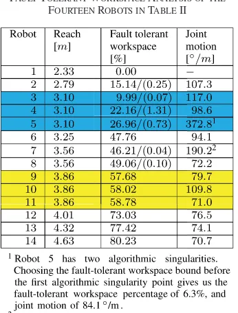
TABLE III
FAULT-TOLERANTWORKSPACEANALYSIS OF THE
FOURTEENROBOTS INTABLEII
fault-tolerant workspace is shown in the last column. Note that Robots
5 and 7 have much larger values for this measure because these robots
encounter algorithmic singularities within the workspace that require
a significant amount of reconfiguration for the robot to stay at the
maximum value of
K
. Robots 2, 3, 4, 5, 7, and 8 have the fault-tolerant
workspace separated into two pieces, i.e., there is a region in between
where the maximum of
K
drops below the optimal value. (Similar is
to that of Robot 3 in the 3R case shown in Fig. 2.) The amount of this
drop varies depending upon the robot, ranging from as small as 0.2%
for Robots 4 and 8, to as large as 9% for Robot 3. The number between
parentheses is the smaller of the two fault-tolerant workspaces, which
in all cases includes the design point.
Clearly, the maximum reach (or sum of the link lengths) has a
dominant effect on the global fault-tolerant properties.
3However, there
are three cases where the same maximum reach can be obtained by
multiple different robot designs with significant differences in their
global fault-tolerant properties. Consider first the case of Robots 9–11.
Even though their fault-tolerant workspace percentages are almost the
same, there is a significant difference in the amount of joint motion
needed to maintain a fault-tolerant configuration. In particular, Robot
3It is important to note that one can always scale these robot designs to obtain
any desired maximum reach, which is why we normalize the fault-tolerant workspace results in Table III to be a percentage.
Fig. 6. Three different configurations with maximumKat three different points along thex-axis trajectory for Robots 9–11. In all cases, the first configu-ration is from the design point at a distance of1/√2, and the last configuration is at the boundary of the fault-tolerant workspace at a distance of approximately three.
11 only moves a total of 177 degrees to traverse the entire fault-tolerant
region, whereas Robots 9 and 10 take 191 and 263 degrees, respectively,
to do so. This is visually illustrated in Fig. 6 where for each robot
three different optimal configurations are shown. (The blue one is at
the design point, the green one is at a boundary of the fault-tolerant
workspace, and the red configuration is at the middle.) Furthermore, the
joint motion is distributed differently for the three robots, with Robot
9 requiring much less motion in joint one, which may be desirable due
to the large moment of inertia associated with this joint.
Robots 3–5 also represent a group with equal reach but different
global properties. If one only considers percentage of fault-tolerant
workspace, then Robot 3 is the worst (at 10%), and Robot 5 is the best
(at 27%). However, Robot 5 encounters two algorithmic singularities
within this region, which require the robot to reconfigure itself to a
new posture in order to maintain
K
at its maximum value. This results
in excessive joint motion over a very short period of time. If one opts
to avoid this reconfiguration and follows the locally optimal value of
K
, then
K
will monotonically decrease and results in a fault-tolerant
workspace percentage of only 6.3%. This is illustrated in Fig. 7. Thus,
one could argue that Robot 4 is the best design out of the three.
VI. E
IGHTD
EGREE-
OF-F
REEDOMM
ANIPULATORE
XAMPLEIn this section, we present the design of a locally optimal eight
degree-of-freedom manipulator operating in a fully six-dimensional
task space in order to illustrate the generality of our approach. An
example of an optimally failure tolerant Jacobian for such a manipulator
is given by (18) at the bottom of the page. This Jacobian satisfies the
optimality equation (4) and is isotropic with equal singular values of
σ
=
n/
3 =
8
/
3
(19)
J
=
⎡
⎢
⎢
⎢
⎢
⎢
⎢
⎢
⎢
⎣
0
0.6865
−
0.1131
0.2439
0.9231
−
0.3824
−
0.8152
−
0.6783
1
−
0.7116
0.3662
0.4505
−
0.3829
−
0.4760
−
0.1903
−
0.6432
0
0.1497
−
0.9236
0.8588
−
0.0354
−
0.7919
0.5469
0.3553
0
0.6475
0.4213
0.9106
−
0.1928
0.8022
0.5691
−
0.4861
0
0.6919
0.8595
0.1982
−
0.5402
−
0.5963
−
0.4379
0.7554
1
0.3197
0.2893
−
0.3626
0.8190
−
0.0289
0.6960
0.4396
⎤
⎥
⎥
⎥
⎥
⎥
⎥
⎥
⎥
⎦
Fig. 7. The relationship betweenKand the distance from the base for Robots 3–5. The plot focuses on the behavior near the design point to highlight the difference in this region. Note that the value ofKfor Robot 5 is shown for joint motion that does not include a discontinuity due to an algorithmic singularity. If the discontinuous joint motion is performed, then theKvalue for Robot 5 is comparable to that of Robot 4.
TABLE IV
DH PARAMETERS OF THEROBOT WHOSEJACOBIAN IS GIVEN BY(18)
and an optimal worst-case failure tolerance of
f
σ
6
=
8
/
3
·
2
/
8 =
2
/
3
.
(20)
The DH parameters of this robot are given in Table IV. One way of
realizing this robot at the design point is shown in Fig. 8. If one performs
a global analysis as described above, the end-effector can be moved
away from the design point a distance of 2.3 m and maintain a
K
value
that is
90
% of the optimal. This configuration is illustrated in Fig. 9.
As is in the planar case, one can perform various operations on this
manipulator Jacobian to obtain different corresponding robots that still
have the property of optimal fault tolerance at the design point.
Conse-quently, the designer has a significant amount of freedom in choosing
the robot geometry. For example, permuting the columns of (18) would
result in an optimally fault-tolerant Jacobian that corresponds to a
dif-ferent manipulator. However, portions of the DH table corresponding to
the modified Jacobian may reappear from the original DH table when
three or more successive columns of the original Jacobian appear in
that order. In this case, the manipulators will share some similarities in
geometry. Unlike the planar case, multiplying a column of the Jacobian
by
−
1
only changes the direction of the corresponding axis of rotation
and does not essentially change the robot geometry.
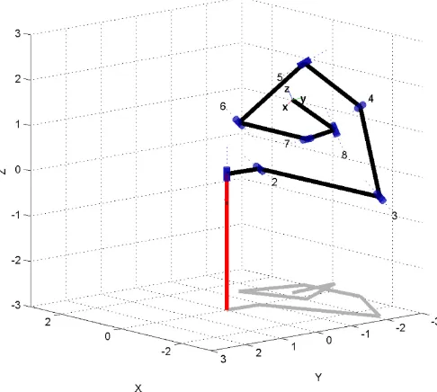
Fig. 8. The eight degree-of-freedom robot that is given in Table IV. This configuration corresponds to the design point for the optimal failure tolerant Jacobian given in (18).4
Fig. 9. The configuration of the eight degree-of-freedom robot that hasKat 90% of the optimalKvalue, which occurs with the end-effector position 2.3 m away from the design point.4
VII. C
ONCLUSIONIt has been previously shown that there are multiple different robot
designs that possess the same desired Jacobian at a specific operating
point. This work has presented a mathematical analysis, based on the
Gram matrix, that allows one to enumerate all of the possible
pla-nar manipulators that possess certain desired fault tolerance properties
based on the form of a desired Jacobian. This analysis was illustrated
on both a 3R manipulator experiencing a single locked joint failure and
a 4R manipulator experiencing two joint failures. It was further shown
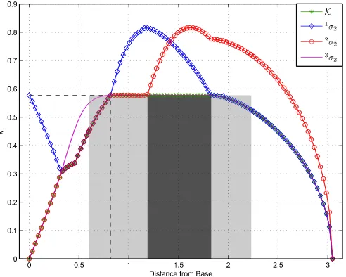
Fig. 10. The relationship betweenKand the distance from the base for Robot 2 in Table I. The minimum singular values for all possible failures are shown for the configuration that maximizesK. Note that if onlyK3were being optimized, then it would be constant for a larger range.
that there are significant differences in the capabilities of the resulting
manipulators, both in terms of pre- and pos-tfailure performance. It
was shown that some of these differences are related to the fact that
the same Jacobian can result in manipulators that vary significantly in
workspace area. However, it is quite surprising that major differences
in behavior were also found in manipulator designs that were identical
in terms of area.
A
PPENDIXE
XPLANATION OFW
HYK
ISC
ONSTANT FORR
OBOT2
INF
IG. 4
A striking feature of Fig. 4 is the flat region of the plot of
K
for
Robot 2. In this Appendix, it will be shown that the maximum value of
3σ
2
for Robot 2 is actually constant for a range of distances from the
base that includes the flat region in Fig. 4. In the case of the analysis
for Robot 2 in Fig. 4, the critical failure happens to be joint 3 over the
region where
K
is flat (see Fig. 10).
We begin by noting that the singular values of the reduced Jacobian
3
J
=
are equal to the square roots of the eigenvalues of
(
3J
)
T(
3J
) =
which are readily given by the characteristic equation of (A2). In
particular, the minimum singular value
3σ
2
of (A1) is given by the
a
1, which together imply that
j
1·
j
2=
The expression for (A3) can then be written as
2(
3σ
2
)
2=
z
+
d
2−
(
z
−
d
2)
2+ (
z
+
d
2−
a
21
)
2(A5)
where, for convenience, we have introduced the notation
z
=
j
22.
Since the link length
a
1is fixed, we have that, for a specified
end-effector distance
d
, (A5) is a function of the single variable
z
, which
we shall denote by
g
(
z
)
.
Setting the derivative of
g
(
z
) =
z
+
d
2−
(
z
−
d
2)
2+ (
z
+
d
2−
a
21
)
2(A6)
to zero, one obtains a single extremal point whose value depends on
whether
d
is greater than, less than, or equal to
a
1/
√
1
, regardless of the specific value
of
d
. For the robot to achieve
z
=
j
22=
d
2, it is necessary and
suf-ficient that
|
a
2−
a
3| ≤
d
≤
a
2+
a
3due to the geometric constraints
on
j
2associated with the lengths of the second and third links. In
summary, if
d > a
1/
2
over all configurations where the end effector is at a distance
d
from the base. It is interesting to note that this solution corresponds
to the end effector being equally distant from the base and the second
joint. Depending on the values of
d
and the link lengths
a
i, these
con-ditions may or may not be possible due to the geometry of the robot. In
the case of Robot 2,
a
1/
[1] K. N. Groom, A. A. Maciejewski, and V. Balakrishnan, “Real-time failure-tolerant control of kinematically redundant manipulators,”IEEE Trans. Robot. Autom., vol. 15, no. 6, pp. 1109–1116, Dec. 1999.
[2] Reliability Information Analysis Center, “Nonelectronic parts reliability data,”Defense Tech. Inform. Center/Air Force Res. Lab, Rome, NY, USA, no. NPRD-2011, 2011.
[3] B. S. Dhillon A. R. M. Fashandi and K. L. Liu, “Robot systems reliability and safety: A review,”J. Quality Maintenance Eng., vol. 8, no. 3, pp. 170– 212, 2002.
[4] H. Nakata, “Domestic robots failed to ride to rescue after No. 1 plant blew,”Japan Times, Jan. 6, 2012.
[5] E. C. Wu, J. C. Hwang, and J. T. Chladek, “Fault-tolerant joint devel-opment for the space shuttle remote manipulator system: Analysis and experiment,”IEEE Trans. Robot. Autom., vol. 9, no. 5, pp. 675–684, Oct. 1993.
[6] G. Visentin and F. Didot, “Testing space robotics on the Japanese ETS-VII satellite,”ESA Bulletin-Eur. Space Agency, vol. 99, pp. 61–65, Sep. 1999. [7] P. S. Babcock and J. J. Zinchuk, “Fault-tolerant design optimization: Ap-plication to an autonomous underwater vehicle navigation system,” in
Proc. Symp. Auton. Underwater Vehicle Technol., Washington, D.C., USA, Jun. 5–6, 1990, pp. 34–43.
[8] R. Colbaugh and M. Jamshidi, “Robot manipulator control for hazardous waste-handling applications,”J. Robot. Syst., vol. 9, no. 2, pp. 215–250, 1992.
[9] W. H. McCulloch, “Safety analysis requirements for robotic systems in DOE nuclear facilities,” inProc. 2nd Specialty Conf. Robot. Challenging Environ., Albuquerque, NM, USA, Jun. 1–6, 1996, pp. 235–240. [10] D. L. Schneider, D. Tesar, and J. W. Barnes, “Development & testing of a
reliability performance index for modular robotic systems,” inProc. Annu. Rel. Maintain. Symp., Anaheim, CA, USA, Jan. 24–27, 1994, pp. 263–271. [11] C. J. J. Paredis and P. K. Khosla, “Designing fault-tolerant manipulators: How many degrees of freedom?,” Int. J. Robot. Res., vol. 15, no. 6, pp. 611–628, Dec. 1996.
[13] C. Carreras and I. D. Walker, “Interval methods for fault-tree analysis in robotics,”IEEE Trans. Robot. Autom., vol. 50, no. 1, pp. 3–11, Mar. 2001. [14] M. L. Visinsky, J. R. Cavallaro, and I. D. Walker, “A dynamic fault toler-ance framework for remote robots,”IEEE Trans. Robot. Autom., vol. 11, no. 4, pp. 477–490, Aug. 1995.
[15] L. Notash, “Joint sensor fault detection for fault tolerant parallel manipu-lators,”J. Robot. Syst., vol. 17, no. 3, pp. 149–157, 2000.
[16] M. Leuschen, I. Walker, and J. Cavallaro, “Fault residual generation via nonlinear analytical redundancy,”IEEE Trans. Control Syst. Tech., vol. 13, no. 3, pp. 452–458, May 2005.
[17] M. Anand, T. Selvaraj, S. Kumanan, and J. Janarthanan, “A hybrid fuzzy logic artificial neural network algorithm-based fault detection and isolation for industrial robot manipulators,”Int. J. Manuf. Res., vol. 2, no. 3, pp. 279–302, 2007.
[18] D. Brambilla, L. Capisani, A. Ferrara, and P. Pisu, “Fault detection for robot manipulators via second-order sliding modes,”IEEE Trans. Ind. Electron., vol. 55, no. 11, pp. 3954–3963, Nov. 2008.
[19] J. Park, W.-K. Chung, and Y. Youm, “Failure recovery by exploiting kine-matic redundancy,” inProc. 5th Int. Workshop Robot Human Commun., Tsukuba, Japan, Nov. 11–14, 1996, pp. 298–305.
[20] X. Chen and S. Nof, “Error detection and prediction algorithms: Appli-cation in robotics,”J. Intell. Robot. Syst.; Robot. Syst., vol. 48, no. 2, pp. 225–252, 2007.
[21] M. Ji and N. Sarkar, “Supervisory fault adaptive control of a mobile robot and its application in sensor-fault accommodation,”IEEE Trans. Robot., vol. 23, no. 1, pp. 174–178, Feb. 2007.
[22] A. De Luca and L. Ferrajoli, “A modified NewtonEuler method for dy-namic computations in robot fault detection and control,” inProc. IEEE Int. Conf. Robot. Autom., May 2009, pp. 3359–3364.
[23] Y. Ting, S. Tosunoglu, and B. Fernandez, “Control algorithms for fault-tolerant robots,” inProc. IEEE Int. Conf. Robot. Autom., May 8–13, 1994, vol. 2, pp. 910–915.
[24] J. D. English and A. A. Maciejewski, “Fault tolerance for kinematically redundant manipulators: Anticipating free-swinging joint failures,”IEEE Trans. Robot. Autom., vol. 14, no. 4, pp. 566–575, Aug. 1998.
[25] J. D. English and A. A. Maciejewski, “Failure tolerance through active braking: A kinematic approach,”Int. J. Robot. Res., vol. 20, no. 4, pp. 287– 299, Apr. 2001.
[26] P. Nieminen, S. Esque, A. Muhammad, J. Mattila, J. V¨ayrynen, M. Siuko, and M. Vilenius, “Water hydraulic manipulator for fail safe and fault tolerant remote handling operations at ITER,”Fusion Eng. Design, vol. 84, no. 7, pp. 1420–1424, 2009.
[27] J. E. McInroy, J. F. O’Brien, and G. W. Neat, “Precise, fault-tolerant point-ing uspoint-ing a Stewart platform,”IEEE/ASME Trans. Mechatronics, vol. 4, no. 1, pp. 91–95, Mar. 1999.
[28] M. Hassan and L. Notash, “Optimizing fault tolerance to joint jam in the design of parallel robot manipulators,”Mech. Mach. Theory, vol. 42, no. 10, pp. 1401–1417, 2007.
[29] Y. Chen, J. E. McInroy, and Y. Yi, “Optimal, fault-tolerant mappings to achieve secondary goals without compromising primary performance,”
IEEE Trans. Robot., vol. 19, no. 4, pp. 680–691, Aug. 2003.
[30] Y. Yi, J. E. McInroy, and Y. Chen, “Fault tolerance of parallel manipulators using task space and kinematic redundancy,”IEEE Trans. Robot., vol. 22, no. 5, pp. 1017–1021, Oct. 2006.
[31] J. E. McInroy and F. Jafari, “Finding symmetric orthogonal Gough– Stewart platforms,”IEEE Trans. Robot., vol. 22, no. 5, pp. 880–889, Oct. 2006.
[32] C. L. Lewis and A. A. Maciejewski, “Dexterity optimization of kinemati-cally redundant manipulators in the presence of failures,”Comput. Electr. Eng.: Int. J., vol. 20, no. 3, pp. 273–288, May 1994.
[33] A. A. Maciejewski, “Fault tolerant properties of kinematically redundant manipulators,” inProc. IEEE Int. Conf. Robot. Autom., Cincinnati, OH, USA, May 13–18, 1990, pp. 638–642.
[34] R. G. Roberts and A. A. Maciejewski, “A local measure of fault tolerance for kinematically redundant manipulators,”IEEE Trans. Robot. Autom., vol. 12, no. 4, pp. 543–552, Aug. 1996.
[35] R. G. Roberts, “On the local fault tolerance of a kinematically redundant manipulator,”J. Robot. Syst., vol. 13, no. 10, pp. 649–661, Oct. 1996. [36] C. J. J. Paredis and P. K. Khosla, “Fault tolerant task execution through
global trajectory planning,”Rel. Eng. Syst. Safety, vol. 53, pp. 225–235, 1996.
[37] C. L. Lewis and A. A. Maciejewski, “Fault tolerant operation of kine-matically redundant manipulators for locked joint failures,”IEEE Trans. Robot. Autom., vol. 13, no. 4, pp. 622–629, Aug. 1997.
[38] R. S. Jamisola, Jr., A. A. Maciejewski, and R. G. Roberts, “Failure-tolerant path planning for kinematically redundant manipulators anticipat-ing locked-joint failures,”IEEE Trans. Robot., vol. 22, no. 4, pp. 603–612, Aug. 2006.
[39] R. G. Roberts, R. J. Jamisola, Jr., and A. A. Maciejewski, “Identifying the failure-tolerant workspace boundaries of a kinematically redundant manipulator,” inProc. IEEE Int. Conf. Robot. Automat., Rome, Italy, Apr. 10–14, 2007, pp. 4517–4523.
[40] K. M. Ben-Gharbia, R. G. Roberts, and A. A. Maciejewski, “Examples of planar robot kinematic designs from optimally fault-tolerant Jacobians,” inProc. IEEE Int. Conf. Robot. Autom., Shanghai, China, May 9–13, 2011, pp. 4710–4715.
[41] T. Yoshikawa, “Manipulability of robotic mechanisms,”Int. J. Robot. Res., vol. 4, no. 2, pp. 3–9, 1985.
[42] C. A. Klein and B. E. Blaho, “Dexterity measures for the design and control of kinematically redundant manipulators,”Int. J. Robot. Res., vol. 6, no. 2, pp. 72–83, 1987.
[43] C. Klein and T. A. Miklos, “Spatial robotic isotropy,”Int. J. Robot. Res., vol. 10, no. 4, pp. 426–437, 1991.
[44] K. E. Zanganeh and J. Angeles, “Kinematic isotropy and the optimum design of parallel manipulators,”Int. J. Robot. Res., vol. 16, no. 2, pp. 185– 197, Apr. 1997.
[45] A. A. Maciejewski and R. G. Roberts, “On the existence of an opti-mally failure tolerant 7R manipulator Jacobian,”Appl. Math. Comput. Sci., vol. 5, no. 2, pp. 343–357, 1995.
[46] P. I. Corke, “A robotics toolbox for MATLAB,”IEEE Robot. Autom. Mag., vol. 3, no. 1, pp. 2–32, Mar. 1996.
Gossip-Based Centroid and Common Reference Frame
Estimation in Multiagent Systems
Mauro Franceschelli and Andrea Gasparri
Abstract—In this study, the decentralized common reference frame
es-timation problem for multiagent systems in the absence of any common coordinate system is investigated. Each agent is deployed in a 2-D space and can only measure the relative distance of neighboring agents and the angle of their line of sight in its local reference frame; no relative atti-tude measurement is available. Only asynchronous and random pairwise communications are allowed between neighboring agents. The convergence properties of the proposed algorithm are characterized, and its sensitiveness against additive noise on the relative distance measurements is investigated. An experimental validation of the effectiveness of the proposed algorithm is provided.
Index Terms—Consensus, distributed randomized algorithms, gossip,
multiagent systems, sensor network localization.
Manuscript received March 23, 2013; revised July 18, 2013; accepted Novem-ber 12, 2013. Date of publication DecemNovem-ber 13, 2013; date of current version April 1, 2014. This paper was recommended for publication by Associate Editor C. C. Cheah and Editor D. Fox upon evaluation of the reviewers’ comments. This work was supported in part by the funding from the European Union Sev-enth Framework Programme [FP7/2007-2013] under Grant agreement 257462 HYCON2 Network of excellence and in part by the Italian Grant FIRB “Futuro in Ricerca,” project NECTAR “Networked Collaborative Team of Autonomous Robots,” code RBFR08QWUV, funded by the Italian Ministry of Research and Education.
M. Franceschelli is with the Department of Electrical and Electronic Engineering, University of Cagliari, 09123 Cagliari, Italy (e-mail: mauro. [email protected]).
A. Gasparri is with the Department of Engineering, Roma Tre University, Rome 00146, Italy (e-mail: [email protected]).
Color versions of one or more of the figures in this paper are available online at http://ieeexplore.ieee.org.
Digital Object Identifier 10.1109/TRO.2013.2291621