❙
R
EMOTE
S
ENSING AND
I
MAGE
I
NTERPRETATION
❙
R
EMOTE
S
ENSING AND
I
MAGE
I
NTERPRETATION
Seventh Edition
Thomas M. Lillesand,
Emeritus University of Wisconsin—MadisonRalph W. Kiefer,
Emeritus University of Wisconsin—MadisonExecutive Editor Ryan Flahive
Cover Photo Quantum Spatial and Washington State DOT
This book was set in 10/12 New Aster by Laserwords and printed and bound by Courier Westford.
Founded in 1807, John Wiley & Sons, Inc. has been a valued source of knowledge and understanding for more than 200 years, helping people around the world meet their needs and fulfill their aspirations. Our company is built on a foundation of principles that include responsibility to the communities we serve and where we live and work. In 2008, we launched a Corporate Citizenship Initiative, a global effort to address the environmental, social, economic, and ethical challenges we face in our business. Among the issues we are addressing are carbon impact, paper specifications and procurement, ethical conduct within our business and among our vendors, and community and charitable support. For more information, please visit our website: www.wiley.com/go/ citizenship.
Copyright © 2015, 2008 John Wiley & Sons, Inc. All rights reserved. No part of this publication may be reproduced, stored in a retrieval system or transmitted in any form or by any means, electronic, mechanical, photocopying, recording, scanning or otherwise, except as permitted under Sections 107 or 108 of the 1976 United States Copyright Act, without either the prior written permission of the Publisher, or authorization through payment of the appropriate per-copy fee to the Copyright Clearance Center, Inc. 222 Rosewood Drive, Danvers, MA 01923, website www.copyright.com. Requests to the Publisher for permission should be addressed to the Permissions Department, John Wiley & Sons, Inc., 111 River Street, Hoboken, NJ 07030-5774, (201) 748-6011, fax (201) 748-6008, website www.wiley.com/go/permissions.
Evaluation copies are provided to qualified academics and professionals for review purposes only, for use in their courses during the next academic year. These copies are licensed and may not be sold or transferred to a third party. Upon completion of the review period, please return the evaluation copy to Wiley. Return instructions and a free-of-charge return mailing label are available at www.wiley.com/go/returnlabel. If you have chosen to adopt this textbook for use in your course, please accept this book as your complimentary desk copy. Outside of the United States, please contact your local sales representative.
Library of Congress Cataloging-in-Publication Data
Lillesand, Thomas M.
Remote sensing and image interpretation / Thomas M. Lillesand, Ralph W. Kiefer, Jonathan W. Chipman.—Seventh edition.
pages cm
Includes bibliographical references and index. ISBN 978-1-118-34328-9 (paperback)
1. Remote sensing. I. Kiefer, Ralph W. II. Chipman, Jonathan W. III. Title. G70.4.L54 2015
621.36'78—dc23
❙
P
REFACE
This book is designed to be primarily used in two ways: as a textbook in intro-ductory courses in remote sensing and image interpretation and as a reference for the burgeoning number of practitioners who use geospatial information and analy-sis in their work. Rapid advances in computational power and sensor design are allowing remote sensing and its kindred technologies, such as geographic information systems (GIS) and the Global Positioning System (GPS), to play an increasingly important role in science, engineering, resource management, com-merce, and otherfields of human endeavor. Because of the wide range of academic
and professional settings in which this book might be used, we have made this dis-cussion “discipline neutral.” That is, rather than writing a book heavily oriented toward a single field such as business, ecology, engineering, forestry, geography,
geology, urban and regional planning, or water resource management, we approach the subject in such a manner that students and practitioners in any discipline should gain a clear understanding of remote sensing systems and their virtually unlimited applications. In short, anyone involved in geospatial data acquisition and analysis shouldfind this book to be a valuable text and reference.
The world has changed dramatically since the first edition of this book was
published, nearly four decades ago. Students may read this new edition in an ebook format on a tablet or laptop computer whose processing power and user interface are beyond the dreams of the scientists and engineers who pioneered the
use of computers in remote sensing and image interpretation in the 1960s and early 1970s. The book’s readers have diversified as thefield of remote sensing has
become a truly international activity, with countries in Asia, Africa, and Latin America contributing at all levels from training new remote sensing analysts, to using geospatial technology in managing their natural resources, to launching and operating new earth observation satellites. At the same time, the proliferation of high‐resolution image‐based visualization platforms—from Google Earth to Microsoft’s Bing Maps—is in a sense turning everyone with access to the Internet into an“armchair remote‐sensing aficionado.”Acquiring the expertise to produce informed, reliable interpretations of all this newly available imagery, however, takes time and effort. To paraphrase the words attributed to Euclid, there is no royal road to image analysis—developing these skills still requires a solid ground-ing in the principles of electromagnetic radiation, sensor design, digital image pro-cessing, and applications.
This edition of the book strongly emphasizes digital image acquisition and analysis, while retaining basic information about earlier analog sensors and meth-ods (from which a vast amount of archival data exist, increasingly valuable as a source for studies of long‐term change). We have expanded our coverage of lidar systems and of 3D remote sensing more generally, including digital photogram-metric methods such as structure‐from‐motion (SFM). In keeping with the chan-ges sweeping the field today, images acquired from uninhabited aerial system
(UAS) platforms are now included among thefigures and color plates, along with
images from many of the new optical and radar satellites that have been launched since the previous edition was published. On the image analysis side, the continu-ing improvement in computational power has led to an increased emphasis on techniques that take advantage of high‐volume data sets, such as those dealing with neural network classification, object‐based image analysis, change detection, and image time‐series analysis.
While adding in new material (including many new images and color plates) and updating our coverage of topics from previous editions, we have also made some improvements to the organization of the book. Most notably, what was formerly Chapter 4—on visual image interpretation—has been split. Thefirst
sec-tions, dealing with methods for visual image interpretation, have been brought into Chapter 1, in recognition of the importance of visual interpretation through-out the book (and the field). The remainder of the former Chapter 4 has been
moved to the end of the book and expanded into a new, broader review of applica-tions of remote sensing not limited to visual methods alone. In addition, our cover-age of radar and lidar systems has been moved ahead of the chapters on digital image analysis methods and applications of remote sensing.
Despite these changes, we have also endeavored to retain the traditional strengths of this book, which date back to the very first edition. As noted above,
different ways. Some courses may omit certain chapters and use the book in a one‐semester or one‐quarter course; the book may also be used in a two‐course sequence. Others may use this discussion in a series of modular courses, or in a shortcourse/workshop format. Beyond the classroom, the remote sensing practi-tioner willfind this book an enduring reference guide—technology changes con-stantly, but the fundamental principles of remote sensing remain the same. We have designed the book with these different potential uses in mind.
As always, this edition stands upon the shoulders of those that preceded it. Many individuals contributed to thefirst six editions of this book, and we thank
them again, collectively, for their generosity in sharing their time and expertise. In addition, we would like to acknowledge the efforts of all the expert reviewers who have helped guide changes in this edition and previous editions. We thank the reviewers for their comments and suggestions.
Illustration materials for this edition were provided by: Dr. Sam Batzli, USGS WisconsinView program, University of Wisconsin—Madison Space Science and Engineering Center; Ruediger Wagner, Vice President of Imaging, Geospatial Solutions Division and Jennifer Bumford, Marketing and Communications, Leica Geosystems; Philipp Grimm, Marketing and Sales Manager, ILI GmbH; Jan Schoderer, Sales Director UltraCam Business Unit and Alexander Wiechert, Busi-ness Director, Microsoft Photogrammetry; Roz Brown, Media Relations Manager, Ball Aerospace; Rick Holasek, NovaSol; Stephen Lich and Jason Howse, ITRES, Inc.; Qinghua Guo and Jacob Flanagan, UC‐Merced; Dr. Thomas Morrison, Wake Forest University; Dr. Andrea Laliberte, Earthmetrics, Inc.; Dr. Christoph Borel‐Donohue, Research Associate Professor of Engineering Physics, U.S. Air Force Institute of Technology; Elsevier Limited, the German Aerospace Center (DLR), Airbus Defence & Space, the Canadian Space Agency, Leica Geosystems, and the U.S. Library of Congress. Dr. Douglas Bolger, Dartmouth College, and Dr. Julian Fennessy, Giraffe Conservation Foundation, generously contributed to the discussion of wildlife monitoring in Chapter 8, including the giraffe telemetry data used in Figure 8.24. Our particular thanks go to those who kindly shared imagery and information about the Oso landslide in Washington State, including images that ultimately appeared in afigure, a color plate, and the front and back
covers of this book; these sources include Rochelle Higgins and Susan Jackson at Quantum Spatial, Scott Campbell at the Washington State Department of Trans-portation, and Dr. Ralph Haugerud of the U.S. Geological Survey.
Numerous suggestions relative to the photogrammetric material contained in this edition were provided by Thomas Asbeck, CP, PE, PLS; Dr. Terry Keating, CP, PE, PLS; and Michael Renslow, CP, RPP.
We also thank the many faculty, academic staff, and graduate and under-graduate students at Dartmouth College and the University of Wisconsin— Madison who made valuable contributions to this edition, both directly and indirectly.
Finally, we want to encourage you, the reader, to use the knowledge of remote sensing that you might gain from this book to literally make the world a better place. Remote sensing technology has proven to provide numerous scientific,
com-mercial, and social benefits. Among these is not only the efficiency it brings to the
day‐to‐day decision‐making process in an ever‐increasing range of applications, but also the potential this field holds for improving the stewardship of earth’s resources and the global environment. This book is intended to provide a technical foundation for you to aid in making this tremendous potential a reality.
Thomas M. Lillesand Ralph W. Kiefer Jonathan W. Chipman
❙
C
ONTENTS
1
Concepts and Foundations of Remote
Sensing 1
1.1 Introduction 1
1.2 Energy Sources and Radiation Principles 4
1.3 Energy Interactions in the Atmosphere 9
1.4 Energy Interactions with Earth Surface Features 12
1.5 Data Acquisition and Digital Image Concepts 30
1.6 Reference Data 39
1.7 The Global Positioning System and Other Global Navigation Satellite Systems 43
1.8 Characteristics of Remote Sensing Systems 45
1.9 Successful Application of Remote Sensing 49
1.10 Geographic Information Systems (GIS) 52
1.11 Spatial Data Frameworks for GIS and Remote Sensing 57
1.12 Visual Image Interpretation 59
2
Elements of Photographic
Systems 85
2.1 Introduction 85
2.2 Early History of Aerial Photography 86
2.3 Photographic Basics 89
3.9 Determining the Elements of Exterior Orientation of Aerial Photographs 189
5.6 Future Landsat Missions and the Global Earth Observation System of Systems 322
5.7 SPOT-1 to -5 324
5.8 SPOT-6 and -7 336
5.10 Moderate Resolution Systems
5.20 Space Station Remote Sensing 379
5.21 Space Debris 382
6
Microwave and Lidar Sensing 385
6.1 Introduction 385
6.2 Radar Development 386
6.3 Imaging Radar System Operation 389
6.4 Synthetic Aperture Radar 399
6.5 Geometric Characteristics of Radar Imagery 402
6.6 Transmission Characteristics of Radar Signals 409
6.7 Other Radar Image Characteristics 413
6.8 Radar Image Interpretation 417
6.9 Interferometric Radar 435
6.10 Radar Remote Sensing from Space 441
6.11 Seasat-1 and the Shuttle Imaging Radar Missions 443
6.12 Almaz-1 448
6.13 ERS, Envisat, and Sentinel-1 448
6.14 JERS-1, ALOS, and ALOS-2 450
6.15 Radarsat 452
6.16 TerraSAR-X, TanDEM-X, and PAZ 455
6.17 The COSMO-SkyMed Constellation 457
6.18 Other High-Resolution Spaceborne Radar Systems 458
6.19 Shuttle Radar Topography Mission 459
6.20 Spaceborne Radar System Summary 462
6.21 Radar Altimetry 464
6.22 Passive Microwave Sensing 466
6.23 Basic Principles of Lidar 471
6.24 Lidar Data Analysis and
7.7 Image Classification 537
7.8 Supervised Classification 538
7.9 The Classification Stage 540
7.10 The Training Stage 546
7.11 Unsupervised Classification 556
7.12 Hybrid Classification 560
7.13 Classification of Mixed Pixels 562
7.14 The Output Stage and Postclassification Smoothing 568
7.15 Object-Based Classification 570
7.17 Classification Accuracy Assessment 575
7.18 Change Detection 582
7.19 Image Time Series Analysis 587
7.20 Data Fusion and GIS Integration 591
7.21 Hyperspectral Image Analysis 598
8.2 Land Use/Land Cover Mapping 611
8.3 Geologic and Soil Mapping 618
8.4 Agricultural Applications 628
8.5 Forestry Applications 632
8.6 Rangeland Applications 638
8.7 Water Resource Applications 639
8.8 Snow and Ice Applications 649
8.9 Urban and Regional Planning
❙
1
C
ONCEPTS AND
F
OUNDATIONS
OF
R
EMOTE
S
ENSING
1.1 INTRODUCTION
Remote sensing is the science and art of obtaining information about an object, area, or phenomenon through the analysis of data acquired by a device that is not in contact with the object, area, or phenomenon under investigation. As you read these words, you are employing remote sensing. Your eyes are acting as sensors that respond to the light reflected from this page. The“data”your eyes acquire are impulses corresponding to the amount of light reflected from the dark and light
areas on the page. These data are analyzed, or interpreted, in your mental compu-ter to enable you to explain the dark areas on the page as a collection of letcompu-ters forming words. Beyond this, you recognize that the words form sentences, and you interpret the information that the sentences convey.
In many respects, remote sensing can be thought of as a reading process. Using various sensors, we remotely collect data that may be analyzed to obtain informationabout the objects, areas, or phenomena being investigated. The remo-tely collected data can be of many forms, including variations in force distribu-tions, acoustic wave distribudistribu-tions, or electromagnetic energy distributions. For example, a gravity meter acquires data on variations in the distribution of the
force of gravity. Sonar, like a bat’s navigation system, obtains data on variations in acoustic wave distributions. Our eyes acquire data on variations in electro-magnetic energy distributions.
Overview of the Electromagnetic Remote Sensing Process
This book is aboutelectromagneticenergy sensors that are operated from airborne and spaceborne platforms to assist in inventorying, mapping, and monitoring earth resources. These sensors acquire data on the way various earth surface features emit and reflect electromagnetic energy, and these data are analyzed to provide information about the resources under investigation.
Figure 1.1 schematically illustrates the generalized processes and elements involved in electromagnetic remote sensing of earth resources. The two basic pro-cesses involved are data acquisition and data analysis. The elements of the data
acquisition process are energy sources (a), propagation of energy through the
atmosphere (b), energy interactions with earth surface features (c), retransmission of energy through the atmosphere (d), airborne and/or spaceborne sensors (e), resulting in the generation of sensor data in pictorial and/or digital form (f). In short, we use sensors to record variations in the way earth surface features reflect and emit electromagnetic energy. The data analysis process (g) involves examining the data using various viewing and interpretation devices to analyze pictorial data and/or a computer to analyze digital sensor data. Reference data about the resour-ces being studied (such as soil maps, crop statistics, orfield-check data) are used
(a) Sources of energy
(c) Earth surface features (e)
when and where available to assist in the data analysis. With the aid of the refer-ence data, the analyst extracts information about the type, extent, location, and condition of the various resources over which the sensor data were collected. This information is then compiled (h), generally in the form of maps, tables, or digital spatial data that can be merged with other“layers”of information in ageographic
information system (GIS). Finally, the information is presented to users (i), who apply it to their decision-making process.
Organization of the Book
In the remainder of this chapter, we discuss the basic principles underlying the remote sensing process. We begin with the fundamentals of electromagnetic energy and then consider how the energy interacts with the atmosphere and with earth surface features. Next, we summarize the process of acquiring remotely sensed data and introduce the concepts underlying digital imagery formats. We also discuss the role that reference data play in the data analysis procedure and describe how the spatial location of reference data observed in thefield is often
determined using Global Positioning System (GPS) methods. These basics will permit us to conceptualize the strengths and limitations of“real” remote sensing systems and to examine the ways in which they depart from an “ideal” remote sensing system. We then discuss briefly the rudiments of GIS technology and the
spatial frameworks (coordinate systems and datums) used to represent the posi-tions of geographic features in space. Because visual examination of imagery will play an important role in every subsequent chapter of this book, thisfirst chapter
concludes with an overview of the concepts and processes involved in visual inter-pretation of remotely sensed images. By the end of this chapter, the reader should have a grasp of the foundations of remote sensing and an appreciation for the close relationship among remote sensing, GPS methods, and GIS operations.
Chapters 2 and 3 deal primarily with photographic remote sensing. Chapter 2 describes the basic tools used in acquiring aerial photographs, including both analog and digital camera systems. Digital videography is also treated in Chapter 2. Chapter 3 describes the photogrammetric procedures by which precise spatial measurements, maps, digital elevation models (DEMs), orthophotos, and other derived products are made from airphotos.
Discussion of nonphotographic systems begins in Chapter 4, which describes the acquisition of airborne multispectral, thermal, and hyperspectral data. In Chapter 5 we discuss the characteristics of spaceborne remote sensing systems and examine the principal satellite systems used to collect imagery from reflected
Chapter 6 is concerned with the collection and analysis of radar and lidar data. Both airborne and spaceborne systems are discussed. Included in this latter category are such systems as the ALOS, Envisat, ERS, JERS, Radarsat, and ICESat satellite systems.
In essence, from Chapter 2 through Chapter 6, this book progresses from the simplest sensing systems to the more complex. There is also a progression from short to long wavelengths along the electromagnetic spectrum (see Section 1.2). That is, discussion centers on photography in the ultraviolet, visible, and near-infrared regions, multispectral sensing (including thermal sensing using emitted long-wavelength infrared radiation), and radar sensing in the microwave region.
Thefinal two chapters of the book deal with the manipulation, interpretation,
and analysis of images. Chapter 7 treats the subject of digital image processing and describes the most commonly employed procedures through which computer-assisted image interpretation is accomplished. Chapter 8 presents a broad range of applications of remote sensing, including both visual interpretation and computer-aided analysis of image data.
Throughout this book, the International System of Units (SI) is used. Tables are included to assist the reader in converting between SI and units of other mea-surement systems.
Finally, a Works Cited section provides a list of references cited in the text. It is not intended to be a compendium of general sources of additional information. Three appendices provided on the publisher’s website (http://www.wiley.com/ college/lillesand) offer further information about particular topics at a level of detail beyond what could be included in the text itself. Appendix A summarizes the various concepts, terms, and units commonly used in radiation measurement in remote sensing. Appendix B includes sample coordinate transformation and resampling procedures used in digital image processing. Appendix C discusses some of the concepts, terminology, and units used to describe radar signals.
1.2 ENERGY SOURCES AND RADIATION PRINCIPLES
Visible light is only one of many forms of electromagnetic energy. Radio waves, ultraviolet rays, radiant heat, and X-rays are other familiar forms. All this energy is inherently similar and propagates in accordance with basic wave theory. As shown in Figure 1.2, this theory describes electromagnetic energy as traveling in a harmonic, sinusoidal fashion at the “velocity of light” c. The distance from one wave peak to the next is thewavelengthl, and the number of peaks passing afixed
point in space per unit time is the wavefrequency v. From basic physics, waves obey the general equation
c¼vl ð1:1Þ
Because c is essentially a constant 3 3108m=sec, frequency
characterize a wave. In remote sensing, it is most common to categorize electro-magnetic waves by their wavelength location within theelectromagnetic spectrum
(Figure 1.3). The most prevalent unit used to measure wavelength along the spec-trum is themicrometerðmÞ. A micrometer equals 13106m.
Although names (such as “ultraviolet” and “microwave”) are generally assigned to regions of the electromagnetic spectrum for convenience, there is no clear-cut dividing line between one nominal spectral region and the next. Divi-sions of the spectrum have grown from the various methods for sensing each type of radiation more so than from inherent differences in the energy characteristics of various wavelengths. Also, it should be noted that the portions of the Figure 1.2 Electromagnetic wave. Components include a sinusoidal electric waveð ÞE and a similar magnetic waveð ÞM at right angles, both being perpendicular to the direction of propagation.
electromagnetic spectrum used in remote sensing lie along a continuum char-acterized by magnitude changes of many powers of 10. Hence, the use of logarith-mic plots to depict the electromagnetic spectrum is quite common. The “visible” portion of such a plot is an extremely small one, because the spectral sensitivity of the human eye extends only from about 0:4m to approximately 0:7m. The color “blue”is ascribed to the approximate range of 0.4 to 0:5m, “green” to 0.5 to 0:6m, and “red”to 0.6 to 0:7m.Ultraviolet(UV) energy adjoins the blue end of the visible portion of the spectrum. Beyond the red end of the visible region are three different categories ofinfrared(IR) waves:near IR(from 0.7 to 1:3m),mid IR (from 1.3 to 3m; also referred to asshortwave IR orSWIR), andthermal IR
(beyond 3 to 14m, sometimes referred to aslongwave IR). At much longer
wave-lengths (1 mm to 1 m) is themicrowaveportion of the spectrum.
Most common sensing systems operate in one or several of the visible, IR, or microwave portions of the spectrum. Within the IR portion of the spectrum, it should be noted that only thermal-IR energy is directly related to the sensation of heat; near- and mid-IR energy are not.
Although many characteristics of electromagnetic radiation are most easily described by wave theory, another theory offers useful insights into how electro-magnetic energy interacts with matter. This theory—the particle theory—suggests that electromagnetic radiation is composed of many discrete units calledphotons
orquanta. The energy of a quantum is given as
Q¼hv ð1:2Þ
where
Q ¼ energy of a quantum;joules Jð Þ h ¼ Planck’s constant, 6:62631034J sec
v ¼ frequency
We can relate the wave and quantum models of electromagnetic radiation behavior by solving Eq. 1.1 forvand substituting into Eq. 1.2 to obtain
Q¼hc
l ð1:3Þ
Thus, we see that the energy of a quantum is inversely proportional to its wavelength. The longer the wavelength involved, the lower its energy content. This
has important implications in remote sensing from the standpoint that naturally emitted long wavelength radiation, such as microwave emission from terrain fea-tures, is more difficult to sense than radiation of shorter wavelengths, such as
emitted thermal IR energy. The low energy content of long wavelength radiation means that, in general, systems operating at long wavelengths must “view” large areas of the earth at any given time in order to obtain a detectable energy signal.
sources of radiation, although it is of considerably different magnitude and spectral composition than that of the sun. How much energy any object radiates is, among other things, a function of the surface temperature of the object. This property is expressed by theStefan–Boltzmann law, which states that
M¼sT4 ð1:4Þ
where
M ¼ total radiant exitance from the surface of a material;watts Wð Þm2 s ¼ Stefan–Boltzmann constant, 5:66973108W m2K4
T ¼ absolute temperature Kð Þof the emitting material
The particular units and the value of the constant are not critical for the stu-dent to remember, yet it is important to note that the total energy emitted from an object varies asT4 and therefore increases very rapidly with increases in tempera-ture. Also, it should be noted that this law is expressed for an energy source that behaves as a blackbody. A blackbody is a hypothetical, ideal radiator that totally absorbs and reemits all energy incident upon it. Actual objects only approach this ideal. We further explore the implications of this fact in Chapter 4; suffice it to say
for now that the energy emitted from an object is primarily a function of its tem-perature, as given by Eq. 1.4.
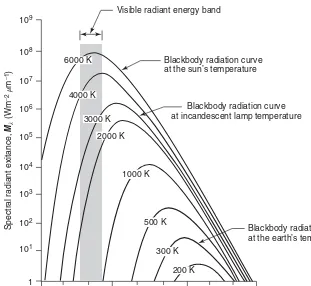
Just as the total energy emitted by an object varies with temperature, the spectral distribution of the emitted energy also varies. Figure 1.4 shows energy distribution curves for blackbodies at temperatures ranging from 200 to 6000 K. The units on the ordinate scale W m 2m1 express the radiant power coming from a blackbody per 1-m spectral interval. Hence, the areaunder these curves
equals the total radiant exitance,M, and the curves illustrate graphically what the
Stefan–Boltzmann law expresses mathematically: The higher the temperature of the radiator, the greater the total amount of radiation it emits. The curves also show that there is a shift toward shorter wavelengths in the peak of a blackbody radiation distribution as temperature increases. The dominant wavelength, or wavelength at which a blackbody radiation curve reaches a maximum, is related to its temperature byWien’s displacement law,
lm¼
A
T ð1:5Þ
where
lm ¼ wavelength of maximum spectral radiant exitance,m
A ¼ 2898mm K T ¼ temperature, K
changes successively to shorter wavelengths—from dull red to orange to yellow and eventually to white.
The sun emits radiation in the same manner as a blackbody radiator whose temperature is about 6000 K (Figure 1.4). Many incandescent lamps emit radia-tion typified by a 3000 K blackbody radiation curve. Consequently, incandescent
lamps have a relatively low output of blue energy, and they do not have the same spectral constituency as sunlight.
The earth’s ambient temperature (i.e., the temperature of surface materials such as soil, water, and vegetation) is about 300 K (27°C). From Wien’s displace-ment law, this means the maximum spectral radiant exitance from earth features occurs at a wavelength of about 9:7m. Because this radiation correlates with terrestrial heat, it is termed“thermal infrared”energy. This energy can neither be seen nor photographed, but it can be sensed with such thermal devices as radio-meters and scanners (described in Chapter 4). By comparison, the sun has a much higher energy peak that occurs at about 0:5m, as indicated in Figure 1.4.
1
Figure 1.4 Spectral distribution of energy radiated from blackbodies of various temperatures. (Note that spectral radiant exitance Ml is the energy emitted per unit wavelength interval.
Our eyes—and photographic sensors—are sensitive to energy of this magnitude and wavelength. Thus, when the sun is present, we can observe earth features by virtue ofreflected solar energy. Once again, the longer wavelength energy emitted
by ambient earth features can be observed only with a nonphotographic sensing system. The general dividing line between reflected and emitted IR wavelengths is
approximately 3m. Below this wavelength, reflected energy predominates; above
it, emitted energy prevails.
Certain sensors, such as radar systems, supply their own source of energy to illuminate features of interest. These systems are termed“active”systems, in con-trast to “passive” systems that sense naturally available energy. A very common example of an active system is a camera utilizing aflash. The same camera used
in sunlight becomes a passive sensor.
1.3 ENERGY INTERACTIONS IN THE ATMOSPHERE
Irrespective of its source, all radiation detected by remote sensors passes through some distance, orpath length, of atmosphere. The path length involved can vary widely. For example, space photography results from sunlight that passes through the full thickness of the earth’s atmosphere twice on its journey from source to sensor. On the other hand, an airborne thermal sensor detects energy emitted directly from objects on the earth, so a single, relatively short atmospheric path length is involved. The net effect of the atmosphere varies with these differences in path length and also varies with the magnitude of the energy signal being sensed, the atmospheric conditions present, and the wavelengths involved.
Because of the varied nature of atmospheric effects, we treat this subject on a sensor-by-sensor basis in other chapters. Here, we merely wish to introduce the notion that the atmosphere can have a profound effect on, among other things, the intensity and spectral composition of radiation available to any sensing sys-tem. These effects are caused principally through the mechanisms of atmospheric
scatteringandabsorption.
Scattering
Atmospheric scattering is the unpredictable diffusion of radiation by particles in the atmosphere.Rayleigh scatter is common when radiation interacts with atmo-spheric molecules and other tiny particles that are much smaller in diameter than the wavelength of the interacting radiation. The effect of Rayleigh scatter is inver-sely proportional to the fourth power of wavelength. Hence, there is a much stronger tendency for short wavelengths to be scattered by this mechanism than long wavelengths.
it scatters the shorter (blue) wavelengths more dominantly than the other visible wavelengths. Consequently, we see a blue sky. At sunrise and sunset, however, the sun’s rays travel through a longer atmospheric path length than during midday. With the longer path, the scatter (and absorption) of short wavelengths is so com-plete that we see only the less scattered, longer wavelengths of orange and red.
Rayleigh scatter is one of the primary causes of “haze” in imagery. Visually, haze diminishes the“crispness,”or“contrast,”of an image. In color photography, it results in a bluish-gray cast to an image, particularly when taken from high alti-tude. As we see in Chapter 2, haze can often be eliminated or at least minimized by introducing, in front of the camera lens, a filter that does not transmit short
wavelengths.
Another type of scatter isMie scatter, which exists when atmospheric particle
diameters essentially equal the wavelengths of the energy being sensed. Water vapor and dust are major causes of Mie scatter. This type of scatter tends to infl
u-ence longer wavelengths compared to Rayleigh scatter. Although Rayleigh scatter tends to dominate under most atmospheric conditions, Mie scatter is significant
in slightly overcast ones.
A more bothersome phenomenon is nonselective scatter, which comes about when the diameters of the particles causing scatter are much larger than the wavelengths of the energy being sensed. Water droplets, for example, cause such scatter. They commonly have a diameter in the range 5 to 100m and scatter all visible and near- to mid-IR wavelengths about equally. Consequently, this scat-tering is “nonselective” with respect to wavelength. In the visible wavelengths, equal quantities of blue, green, and red light are scattered; hence fog and clouds appear white.
Absorption
In contrast to scatter, atmospheric absorption results in the effective loss of energy to atmospheric constituents. This normally involves absorption of energy at a given wavelength. The most efficient absorbers of solar radiation in this
regard are water vapor, carbon dioxide, and ozone. Because these gases tend to absorb electromagnetic energy in specific wavelength bands, they strongly infl
u-ence the design of any remote sensing system. The wavelength ranges in which the atmosphere is particularly transmissive of energy are referred to as atmo-spheric windows.
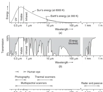
Figure 1.5 shows the interrelationship between energy sources and atmo-spheric absorption characteristics. Figure 1.5a shows the spectral distribution of the energy emitted by the sun and by earth features. These two curves represent the most common sources of energy used in remote sensing. In Figure 1.5b,
“visible”range) coincides with both an atmospheric window and the peak level of energy from the sun. Emitted “heat” energy from the earth, shown by the small curve in (a), is sensed through the windows at 3 to 5m and 8 to 14m using such devices as thermal sensors. Multispectral sensors observe simultaneously through multiple, narrow wavelength ranges that can be located at various points in the visible through the thermal spectral region. Radar andpassive microwave systemsoperate through a window in the region 1 mm to 1 m.
The important point to note from Figure 1.5 is the interaction and the inter-dependence between the primary sources of electromagnetic energy, the atmospheric windows through which source energy may be transmitted to and from earth surface features, and the spectral sensitivity of the sensors available to detect and record the energy. One cannot select the sensor to be used in any given remote sensing task
arbitrarily; one must instead consider (1) the spectral sensitivity of the sensors available, (2) the presence or absence of atmospheric windows in the spectral range(s) in which one wishes to sense, and (3) the source, magnitude, and
(a)
(b)
(c)
spectral composition of the energy available in these ranges. Ultimately, however, the choice of spectral range of the sensor must be based on the manner in which the energy interacts with the features under investigation. It is to this last, very important, element that we now turn our attention.
1.4 ENERGY INTERACTIONS WITH EARTH SURFACE FEATURES
When electromagnetic energy is incident on any given earth surface feature, three fundamental energy interactions with the feature are possible. These are illu-strated in Figure 1.6 for an element of the volume of a water body. Various frac-tions of the energy incident on the element are reflected, absorbed, and/or transmitted. Applying the principle of conservation of energy, we can state the
interrelationship among these three energy interactions as
EIð Þ ¼l ERð Þ þl EAð Þ þl ETð Þl ð1:6Þ
where
EI ¼ incident energy
ER ¼ reflected energy
EA ¼ absorbed energy
ET ¼ transmitted energy
with all energy components being a function of wavelengthl.
Equation 1.6 is an energy balance equation expressing the interrelationship among the mechanisms of reflection, absorption, and transmission. Two points
concerning this relationship should be noted. First, the proportions of energy reflected, absorbed, and transmitted will vary for different earth features,
depend-ing on their material type and condition. These differences permit us to distin-guish different features on an image. Second, the wavelength dependency means that, even within a given feature type, the proportion of reflected, absorbed, and
EI(λ) = Incident energy
ER(λ) = Reflected energy
EA(λ) = Absorbed energy ET(λ) = Transmitted energy
EI(λ) = ER(λ) + EA(λ) + ET(λ)
transmitted energy will vary at different wavelengths. Thus, two features may be indistinguishable in one spectral range and be very different in another wave-length band. Within the visible portion of the spectrum, these spectral variations result in the visual effect called color. For example, we call objects “blue” when they reflect more highly in the blue portion of the spectrum,“green” when they reflect more highly in the green spectral region, and so on. Thus, the eye utilizes
spectral variations in the magnitude of reflected energy to discriminate between
various objects. Color terminology and color mixing principles are discussed fur-ther in Section 1.12.
Because many remote sensing systems operate in the wavelength regions in which reflected energy predominates, the reflectance properties of earth features
are very important. Hence, it is often useful to think of the energy balance rela-tionship expressed by Eq. 1.6 in the form
ERð Þ ¼l EIð Þ l ½EAð Þ þl ETð Þl ð1:7Þ That is, the reflected energy is equal to the energy incident on a given feature
reduced by the energy that is either absorbed or transmitted by that feature. The reflectance characteristics of earth surface features may be quantified by
measuring the portion of incident energy that is reflected. This is measured as a
function of wavelength and is called spectral reflectance, rl. It is mathematically defined as
rl ¼ERð Þl EIð Þl
¼ energy of wavelengthenergy of wavelengthlreflected from the object
lincident upon the object3100 ð1:8Þ whererlis expressed as a percentage.
A graph of the spectral reflectance of an object as a function of wavelength is
termed a spectral reflectance curve. The configuration of spectral reflectance
curves gives us insight into the spectral characteristics of an object and has a strong influence on the choice of wavelength region(s) in which remote sensing
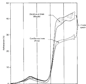
data are acquired for a particular application. This is illustrated in Figure 1.7, which shows highly generalized spectral reflectance curves for deciduous versus
coniferous trees. Note that the curve for each of these object types is plotted as a“ribbon” (or“envelope”) of values, not as a single line. This is because spectral reflectances vary somewhat within a given material class. That is, the spectral
reflectance of one deciduous tree species and another will never be identical, nor
will the spectral reflectance of trees of the same species be exactly equal. We
ela-borate upon the variability of spectral reflectance curves later in this section.
type overlap in most of the visible portion of the spectrum and are very close where they do not overlap. Hence, the eye might see both tree types as being essentially the same shade of“green”and might confuse the identity of the deciduous and con-iferous trees. Certainly one could improve things somewhat by using spatial clues to each tree type’s identity, such as size, shape, site, and so forth. However, this is often difficult to do from the air, particularly when tree types are intermixed. How
might we discriminate the two types on the basis of their spectral characteristics alone? We could do this by using a sensor that records near-IR energy. A specia-lized digital camera whose detectors are sensitive to near-IR wavelengths is just such a system, as is an analog camera loaded with black and white IR film. On
near-IR images, deciduous trees (having higher IR reflectance than conifers)
gen-erally appear much lighter in tone than do conifers. This is illustrated in Figure 1.8, which shows stands of coniferous trees surrounded by deciduous trees. In Figure 1.8a(visible spectrum), it is virtually impossible to distinguish between tree types, even though the conifers have a distinctive conical shape whereas the deciduous trees have rounded crowns. In Figure 1.8b (near IR), the coniferous trees have a Figure 1.7 Generalized spectral reflectance envelopes for deciduous
(a)
(b)
Figure 1.8 Low altitude oblique aerial photographs illustrating deciduous versus coniferous trees. (a) Panchromatic photograph recording reflected sunlight over the wavelength band 0.4 to 0:7m.
(b) Black-and-white infrared photograph recording reflected sunlight over 0.7 to0:9m wavelength band.
distinctly darker tone. On such an image, the task of delineating deciduous versus coniferous trees becomes almost trivial. In fact, if we were to use a computer to analyze digital data collected from this type of sensor, we might “automate” our entire mapping task. Many remote sensing data analysis schemes attempt to do just that. For these schemes to be successful, the materials to be differentiated must be spectrally separable.
Experience has shown that many earth surface features of interest can be iden-tified, mapped, and studied on the basis of their spectral characteristics. Experience
has also shown that some features of interest cannot be spectrally separated. Thus, to utilize remote sensing data effectively, one must know and understand the spec-tral characteristics of the particular features under investigation in any given appli-cation. Likewise, one must know what factors influence these characteristics.
Spectral Re
fl
ectance of Earth Surface Feature Types
Figure 1.9 shows typical spectral reflectance curves for many different types of
features: healthy green grass, dry (non-photosynthetically active) grass, bare soil (brown to dark-brown sandy loam), pure gypsum dune sand, asphalt, construc-tion concrete (Portland cement concrete), fine-grained snow, clouds, and clear
lake water. The lines in this figure represent average reflectance curves compiled
by measuring a large sample of features, or in some cases representative refl
ec-tance measurements from a single typical example of the feature class. Note how distinctive the curves are for each feature. In general, the configuration of these
curves is an indicator of the type and condition of the features to which they apply. Although the reflectance of individual features can vary considerably above
and below the lines shown here, these curves demonstrate some fundamental points concerning spectral reflectance.
For example, spectral reflectance curves for healthy green vegetation almost
always manifest the “peak-and-valley” configuration illustrated by green grass in
Figure 1.9. The valleys in the visible portion of the spectrum are dictated by the pigments in plant leaves. Chlorophyll, for example, strongly absorbs energy in the wavelength bands centered at about 0.45 and 0:67m (often called the “ chlor-ophyll absorption bands”). Hence, our eyes perceive healthy vegetation as green in color because of the very high absorption of blue and red energy by plant leaves and the relatively high reflection of green energy. If a plant is subject to
some form of stress that interrupts its normal growth and productivity, it may decrease or cease chlorophyll production. The result is less chlorophyll absorp-tion in the blue and red bands. Often, the red reflectance increases to the point
that we see the plant turn yellow (combination of green and red). This can be seen in the spectral curve for dried grass in Figure 1.9.
As we go from the visible to the near-IR portion of the spectrum, the refl
Figure 1.9 Spectral reflectance curves for various features types. (Original data courtesy USGS
Spectroscopy Lab, Johns Hopkins University Spectral Library, and Jet Propulsion Laboratory [JPL]; cloud spectrum from Bowker et al., after Avery and Berlin, 1992. JPL spectra © 1999, California Institute of Technology.)
0.75 to 1:3m (representing most of the near-IR range), a plant leaf typically reflects 40 to 50% of the energy incident upon it. Most of the remaining energy is
plant leaves. Because the position of the red edge and the magnitude of the near-IR reflectance beyond the red edge are highly variable among plant species, reflectance
measurements in these ranges often permit us to discriminate between species, even if they look the same in visible wavelengths. Likewise, many plant stresses alter the reflectance in the red edge and the near-IR region, and sensors operating
in these ranges are often used for vegetation stress detection. Also, multiple layers of leaves in a plant canopy provide the opportunity for multiple transmissions and reflections. Hence, the near-IR reflectance increases with the number of layers of
leaves in a canopy, with the maximum reflectance achieved at about eight leaf
layers (Bauer et al., 1986).
Beyond 1:3m, energy incident upon vegetation is essentially absorbed or reflected, with little to no transmittance of energy. Dips in reflectance occur at
1.4, 1.9, and 2:7m because water in the leaf absorbs strongly at these wave-lengths. Accordingly, wavelengths in these spectral regions are referred to as
water absorption bands. Reflectance peaks occur at about 1.6 and 2:2m,
between the absorption bands. Throughout the range beyond 1:3m, leaf reflectance is approximately inversely related to the total water present in a
leaf. This total is a function of both the moisture content and the thickness of a leaf.
The soil curve in Figure 1.9 shows considerably less peak-and-valley variation in reflectance. That is, the factors that influence soil reflectance act over less
spe-cific spectral bands. Some of the factors affecting soil reflectance are moisture
content, organic matter content, soil texture (proportion of sand, silt, and clay), surface roughness, and presence of iron oxide. These factors are complex, vari-able, and interrelated. For example, the presence of moisture in soil will decrease its reflectance. As with vegetation, this effect is greatest in the water absorption
bands at about 1.4, 1.9, and 2:7m (clay soils also have hydroxyl absorption bands at about 1.4 and 2:2m). Soil moisture content is strongly related to the soil texture: Coarse, sandy soils are usually well drained, resulting in low moisture content and relatively high reflectance; poorly drained fine-textured soils will
generally have lower reflectance. Thus, the reflectance properties of a soil are
con-sistent only within particular ranges of conditions. Two other factors that reduce soil reflectance are surface roughness and content of organic matter. The
pre-sence of iron oxide in a soil will also significantly decrease reflectance, at least in
the visible wavelengths. In any case, it is essential that the analyst be familiar with the conditions at hand. Finally, because soils are essentially opaque to visi-ble and infrared radiation, it should be noted that soil reflectance comes from the
uppermost layer of the soil and may not be indicative of the properties of the bulk of the soil.
Sand can have wide variation in its spectral reflectance pattern. The curve
material, gypsum. Sand derived from other sources, with differing mineral com-positions, would have a spectral reflectance curve indicative of its parent
mate-rial. Other factors affecting the spectral response from sand include the presence or absence of water and of organic matter. Sandy soil is subject to the same con-siderations listed in the discussion of soil reflectance.
As shown in Figure 1.9, the spectral reflectance curves for asphalt and
Port-land cement concrete are muchflatter than those of the materials discussed thus
far. Overall, Portland cement concrete tends to be relatively brighter than asphalt, both in the visible spectrum and at longer wavelengths. It is important to note that the reflectance of these materials may be modified by the presence of
paint, soot, water, or other substances. Also, as materials age, their spectral reflectance patterns may change. For example, the reflectance of many types of
asphaltic concrete may increase, particularly in the visible spectrum, as their sur-face ages.
In general, snow reflects strongly in the visible and near infrared, and absorbs
more energy at mid-infrared wavelengths. However, the reflectance of snow is
affected by its grain size, liquid water content, and presence or absence of other materials in or on the snow surface (Dozier and Painter, 2004). Larger grains of snow absorb more energy, particularly at wavelengths longer than 0:8m. At tem-peratures near 0°C, liquid water within the snowpack can cause grains to stick together in clusters, thus increasing the effective grain size and decreasing the reflectance at near-infrared and longer wavelengths. When particles of
con-taminants such as dust or soot are deposited on snow, they can significantly reduce
the surface’s reflectance in the visible spectrum.
The aforementioned absorption of mid-infrared wavelengths by snow can per-mit the differentiation between snow and clouds. While both feature types appear bright in the visible and near infrared, clouds have significantly higher reflectance
than snow at wavelengths longer than 1:4m. Meteorologists can also use both spectral and bidirectional reflectance patterns (discussed later in this section) to
identify a variety of cloud properties, including ice/water composition and particle size.
Considering the spectral reflectance of water, probably the most distinctive
characteristic is the energy absorption at near-IR wavelengths and beyond. In short, water absorbs energy in these wavelengths whether we are talking about water features per se (such as lakes and streams) or water contained in vegetation or soil. Locating and delineating water bodies with remote sensing data are done most easily in near-IR wavelengths because of this absorption property. However, various conditions of water bodies manifest themselves pri-marily in visible wavelengths. The energy–matter interactions at these wave-lengths are very complex and depend on a number of interrelated factors. For example, the reflectance from a water body can stem from an interaction with
the water’s surface (specular reflection), with material suspended in the water,
deep water where bottom effects are negligible, the reflectance properties of a
water body are a function of not only the water per se but also the material in the water.
Clear water absorbs relatively little energy having wavelengths less than about 0:6m. High transmittance typifies these wavelengths with a maximum in
the blue-green portion of the spectrum. However, as the turbidity of water chan-ges (because of the presence of organic or inorganic materials), transmittance— and therefore reflectance—changes dramatically. For example, waters containing large quantities of suspended sediments resulting from soil erosion normally have much higher visible reflectance than other “clear” waters in the same geo-graphic area. Likewise, the reflectance of water changes with the chlorophyll
concentration involved. Increases in chlorophyll concentration tend to decrease water reflectance in blue wavelengths and increase it in green wavelengths.
These changes have been used to monitor the presence and estimate the con-centration of algae via remote sensing data. Reflectance data have also been used
to determine the presence or absence of tannin dyes from bog vegetation in lowland areas and to detect a number of pollutants, such as oil and certain industrial wastes.
Figure 1.10 illustrates some of these effects, using spectra from three lakes with different bio-optical properties. The first spectrum is from a clear,
oligo-trophic lake with a chlorophyll level of 1:2g=l and only 2.4 mg/l of dissolved organic carbon (DOC). Its spectral reflectance is relatively high in the blue-green
portion of the spectrum and decreases in the red and near infrared. In contrast,
Figure 1.10 Spectral reflectance curves for lakes with clear water, high levels of
the spectrum from a lake experiencing an algae bloom, with much higher chlor-ophyll concentration 12ð :3g=lÞ, shows a reflectance peak in the green spectrum
and absorption in the blue and red regions. These reflectance and absorption
fea-tures are associated with several pigments present in algae. Finally, the third spectrum in Figure 1.10 was acquired on an ombrotrophic bog lake, with very high levels of DOC (20.7 mg/l). These naturally occurring tannins and other com-plex organic molecules give the lake a very dark appearance, with its reflectance
curve nearlyflat across the visible spectrum.
Many important water characteristics, such as dissolved oxygen concentra-tion, pH, and salt concentraconcentra-tion, cannot be observed directly through changes in water reflectance. However, such parameters sometimes correlate with
observed reflectance. In short, there are many complex interrelationships
between the spectral reflectance of water and particular characteristics. One
must use appropriate reference data to correctly interpret reflectance
measure-ments made over water.
Our discussion of the spectral characteristics of vegetation, soil, and water has been very general. The student interested in pursuing details on this subject, as well as factors influencing these characteristics, is encouraged to consult the
various references contained in the Works Cited section located at the end of this book.
Spectral Response Patterns
Having looked at the spectral reflectance characteristics of vegetation, soil, sand,
concrete, asphalt, snow, clouds, and water, we should recognize that these broad feature types are often spectrally separable. However, the degree of separation between types varies among and within spectral regions. For example, water and vegetation might reflect nearly equally in visible wavelengths, yet these features
are almost always separable in near-IR wavelengths.
Because spectral responses measured by remote sensors over various features often permit an assessment of the type and/or condition of the features, these responses have often been referred to as spectral signatures. Spectral reflectance
and spectral emittance curves (for wavelengths greater than 3:0m) are often referred to in this manner. The physical radiation measurements acquired over specific terrain features at various wavelengths are also referred to as the spectral
signatures for those features.
Although it is true that many earth surface features manifest very distinctive spectral reflectance and/or emittance characteristics, these characteristics result
in spectral“response patterns”rather than in spectral“signatures.”The reason for this is that the termsignaturetends to imply a pattern that is absolute and unique.
quantitative, but they are not absolute. They may be distinctive, but they are not necessarily unique.
We have already looked at some characteristics of objects that influence their
spectral response patterns. Temporal effectsandspatial effectscan also enter into any given analysis. Temporal effects are any factors that change the spectral char-acteristics of a feature over time. For example, the spectral charchar-acteristics of many species of vegetation are in a nearly continual state of change throughout a growing season. These changes often influence when we might collect sensor data
for a particular application.
Spatial effects refer to factors that cause the same types of features (e.g., corn plants) at a given point intime to have different characteristics at different
geo-graphic locations. In small-area analysis the geographic locations may be meters
apart and spatial effects may be negligible. When analyzing satellite data, the locations may be hundreds of kilometers apart where entirely different soils, cli-mates, and cultivation practices might exist.
Temporal and spatial effects influence virtually all remote sensing operations.
These effects normally complicate the issue of analyzing spectral reflectance
properties of earth resources. Again, however, temporal and spatial effects might be the keys to gleaning the information sought in an analysis. For example, the process ofchange detectionis premised on the ability to measure temporal effects. An example of this process is detecting the change in suburban development near a metropolitan area by using data obtained on two different dates.
An example of a useful spatial effect is the change in the leaf morphology of trees when they are subjected to some form of stress. For example, when a tree becomes infected with Dutch elm disease, its leaves might begin to cup and curl, changing the reflectance of the tree relative to healthy trees that surround it. So,
even though a spatial effect might cause differences in the spectral reflectances of
the same type of feature, this effect may be just what is important in a particular application.
Finally, it should be noted that the apparent spectral response from surface features can be influenced by shadows. While an object’s spectral reflectance
(a ratio of reflected to incident energy, see Eq. 1.8) is not affected by changes in
illumination, the absolute amount of energy reflected does depend on
illumina-tion condiillumina-tions. Within a shadow, the total reflected energy is reduced, and the
spectral response is shifted toward shorter wavelengths. This occurs because the incident energy within a shadow comes primarily from Rayleigh atmospheric scattering, and as discussed in Section 1.3, such scattering primarily affects short wavelengths. Thus, in visible-wavelength imagery, objects inside shadows will tend to appear both darker and bluer than if they were fully illuminated. This effect can cause problems for automated image classification algorithms; for
example, dark shadows of trees on pavement may be misclassified as water. The
effects of illumination geometry on reflectance are discussed in more detail later
Atmospheric In
fl
uences on Spectral Response Patterns
In addition to being influenced by temporal and spatial effects, spectral response
patterns are influenced by the atmosphere. Regrettably, the energy recorded by a
sensor is always modified to some extent by the atmosphere between the sensor
and the ground. We will indicate the significance of this effect on a
sensor-by-sensor basis throughout this book. For now, Figure 1.11 provides an initial frame of reference for understanding the nature of atmospheric effects. Shown in this
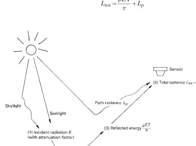
figure is the typical situation encountered when a sensor records reflected solar
energy. The atmosphere affects the “brightness,” or radiance, recorded over any given point on the ground in two almost contradictory ways. First, it attenuates (reduces) the energy illuminating a ground object (and being reflected from the
object). Second, the atmosphere acts as a reflector itself, adding a scattered,
extra-neouspath radianceto the signal detected by the sensor. By expressing these two
atmospheric effects mathematically, the total radiance recorded by the sensor may be related to the reflectance of the ground object and the incoming radiation
orirradianceusing the equation
Ltot¼rET
þLp ð1:9Þ
Figure 1.11 Atmospheric effects influencing the measurement of reflected solar energy.
Attenuated sunlight and skylightð ÞE is reflected from a terrain element having reflectancer. The
attenuated radiance reflected from the terrain elementðrET=Þcombines with the path radiance
Lp
where
Ltot ¼ total spectral radiance measured by sensor
r ¼ reflectance of object
E ¼ irradiance on object;incoming energy
T ¼ transmission of atmosphere
Lp ¼ path radiance;from the atmosphere and not from the object
It should be noted that all of the above factors depend on wavelength. Also, as shown in Figure 1.11, the irradianceð ÞE stems from two sources: (1) directly refl ec-ted“sunlight”and (2) diffuse“skylight,” which is sunlight that has been previously scattered by the atmosphere. The relative dominance of sunlight versus skylight in any given image is strongly dependent on weather conditions (e.g., sunny vs. hazy vs. cloudy). Likewise, irradiance varies with the seasonal changes in solar elevation angle (Figure 7.4) and the changing distance between the earth and sun.
For a sensor positioned close to the earth’s surface, the path radianceLp will generally be small or negligible, because the atmospheric path length from the surface to the sensor is too short for much scattering to occur. In contrast, ima-gery from satellite systems will be more strongly affected by path radiance, due to the longer atmospheric path between the earth’s surface and the spacecraft. This can be seen in Figure 1.12, which compares two spectral response patterns from the same area. One“signature”in thisfigure was collected using a handheld field spectroradiometer (see Section 1.6 for discussion), from a distance of only a few cm above the surface. The second curve shown in Figure 1.12 was collected by the Hyperion hyperspectral sensor on the EO-1 satellite (hyperspectral systems
0.4 0.5 0.6 0.7 0.8 0.9 1
Satellite
Surface
Spectral radiance
Wavelength (μm)
Figure 1.12 Spectral response patterns measured using a field
are discussed in Chapter 4, and the Hyperion instrument is covered in Chapter 5). Due to the thickness of the atmosphere between the earth’s surface and the satel-lite’s position above the atmosphere, this second spectral response pattern shows an elevated signal at short wavelengths, due to the extraneous path radiance.
In its raw form, this near-surface measurement from the field
spectro-radiometer could not be directly compared to the measurement from the satellite, because one is observing surface reflectance while the other is observing the so-called top of atmosphere (TOA) reflectance. Before such a comparison could be
performed, the satellite image would need to go through a process ofatmospheric correction, in which the raw spectral data are modified to compensate for the
expected effects of atmospheric scattering and absorption. This process, discussed in Chapter 7, generally does not produce a perfect representation of the spectral response curve that would actually be observed at the surface itself, but it can pro-duce a sufficiently close approximation to be suitable for many types of analysis.
Readers who might be interested in obtaining additional details about the concepts, terminology, and units used in radiation measurement may wish to consult Appendix A.
Geometric In
fl
uences on Spectral Response Patterns
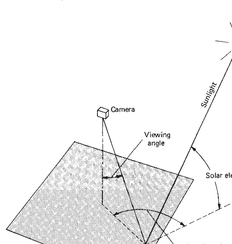
The geometric manner in which an object reflects energy is an important
con-sideration. This factor is primarily a function of the surface roughness of the object. Specular reflectors are flat surfaces that manifest mirror-like reflections,
where the angle of reflection equals the angle of incidence. Diffuse (or Lamber-tian) reflectors are rough surfaces that reflect uniformly in all directions. Most
earth surfaces are neither perfectly specular nor perfectly diffuse reflectors. Their
characteristics are somewhat between the two extremes.
Figure 1.13 illustrates the geometric character of specular, near-specular, near-diffuse, and diffuse reflectors. The category that describes any given surface
is dictated by the surface’s roughness in comparison to the wavelength of the energy being sensed. For example, in the relatively long wavelength radio range, a sandy beach can appear smooth to incident energy, whereas in the visible portion of the spectrum, it appears rough. In short, when the wavelength of incident energy is much smaller than the surface height variations or the particle sizes that make up a surface, the reflection from the surface is diffuse.
Diffuse reflections contain spectral information on the“color”of the reflecting
surface, whereas specular reflections generally do not.Hence, in remote sensing, we are most often interested in measuring the diffuse reflectance properties of terrain features.
Because most features are not perfect diffuse reflectors, however, it becomes
apparent reflectance in an image. In (a), the effect of differential shading is
illu-strated in profile view. Because the sides of features may be either sunlit or
sha-ded, variations in brightness can result from identical ground objects at different locations in the image. The sensor receives more energy from the sunlit side of the tree at B than from the shaded side of the tree at A. Differential shading is
clearly a function of solar elevation and object height, with a stronger effect at Figure 1.13 Specular versus diffuse reflectance. (We are most often interested in measuring the diffuse
reflectance of objects.)

![Figure 1.9Spectral reSpectroscopy Lab, Johns Hopkins University Spectral Library, and Jet Propulsion Laboratory [JPL]; cloudspectrum from Bowker et al., after Avery and Berlin, 1992](https://thumb-ap.123doks.com/thumbv2/123dok/3859697.1841957/31.624.111.472.59.500/spectral-respectroscopy-hopkins-university-spectral-propulsion-laboratory-cloudspectrum.webp)