NUMERICAL STUDY ON THE STABILITY OF
TAKENS-BOGDANOV SYSTEMS
Tulus
Abstract. This paper presents the results of a research performed on a
Takens-Bogdanov equation. The objective is to find the dynamics of the solution with deal to prescribed initial conditions. A fifth order Runge-Kutta method is used, and applied to two cases, i.e. forµ1>0andµ1<0. In the first case, there is no fixed point found. On the other hand, in the second one, there are two fixed points, a stable fixed point and an unstable fixed point.
1. INTRODUCTION
Takens-Bogdanov bifurcation is a dynamical behavior that is not trivial with double-zero eigenvalues of the linearization matrix. It is known that in a versal deformation of Takens-Bogdanov bifurcation, it is possible to find a dynamic system that moves to a saddle point, bifurcation Hopf and homoclinic. Algaba et al. [1] has studied Takens-Bogdanov bifurcation in the Chua equation using cubic non-linearity. On teh other hand, Carillo and Verduzco [2] has considered a nonlinear control system in the plane, which its nominal vector field has some double-zero eigenvalues, and then get the idea of finding that in the condition there exists a law of scalar control such that allows a priori, that the closed loop system moves towards any of the above three bifurcation types.
Received 02-12-2011, Accepted 23-12-2011.
2010 Mathematics Subject Classification: 37M20
Key words and Phrases: Takens-Bogdanov Equations, Runge-Kutta Method, bifurcations.
Runge-Kutta method (RK) is one of the well-known numerical method to solve differential equations and is the most common version is the order 4 and 5. The improvement of this method has also been widely performed. Ababneh et al. [3] has been found RK method with a new multiple step. Meanwhile, Sermutlu [4] used RK method of order 4 and 5 for the Lorenz equations. On the other hand, Adomian decomposition method is used for the Lorenz equations and compare it with the Runge-Kutta of order-4 (RK4). An then also Razali and Ahmad [5] compared the solution between a method that is applied to the chaotic and nonchaotic Lorenz system. In this paper, it will be analyzed the dynamic of the Takens-Bogdanov system by varying the parameters in the system.
2. RUNGE-KUTTA ORDER 5
Let us consider the following ordinary differential equation.
d
dtx1 = f1(x1, x2,· · · , xn, t) d
dtx2 = f2(x1, x2,· · · , xn, t) (1)
.. . ... d
dtxn = fn(x1, x2,· · ·, xn, t)
This equation is a non autonomous equations [4]. If the variable t does not appear on the right hand side of the equation (1), then we have an autonomous equation. If the functionf on the right hand side is non linear, then we need some numerical techniques. A Taylor series can be used to solve a such differential equation. But, the series still need the calculation of its derivatives up to degree ofi,fi. This is in practice difficult. Runge-Kutta method has an accuracy as same as Taylor series, up to specified order. And this method does not need to calculate its derivatives compared to Taylor series.
using the following steps.
. From the theory of normal form, there exist a coordinate transformation such that the original system can be expressed up to second order in the form of
˙
which is called a truncated normal form, and assume that a0b0 6= 0. This
section is to study the family introduced by Guckenheimer and Holmes [6], that is
where µ= (µ1, µ2) express the versal deformation of the truncated system
(3). Carrillo and Verduzco [2] proved that for µ1 = 0 and µ2 6= 0, the
family indicates a system toward to saddle point bifurcation, and then the system leading to Hopf bifurcation forµ1 =−µ22, and also the system have
In this study, it is considered the values a0 = 1 and b0 = 1 for the
system of Takens-Bogdanov, that is
d
system does not have a fixed point forµ >0.
The stability of the fixed point can be checked by using the following technique. The Jacobian of the voctor field evaluated at the fixed points are given by
And the eigen value is given by
λ1,2 =
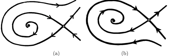
According to [7], when µ2 > 0 and µ1 small negative, then it occurs
the stable and unstable manifold, with a characteristic as depicted in Figure 1. And then, ifµ1 =−µ22 there exist a periodic orbit, as visualize in Figure
2.
Runge-Kutta for Takens-Bogdanov eqution
In this study, the solution of the equation is computed numerically using Runge-Kutta method of order five in two directions, namely the forward direction (by using positive dt) and after that for backward direction (by using negative dt). The first starting point is determined by selecting an arbitrary point in (x1, x2). The next starting point is determined by
(a) (b)
Figure 1: Stable and unstable manifold
Figure 2: Periodic manifold
The time interval used is fromt= 0 until t= 20. The change time dt starts from 0.01, and then changed gradually, with each step dt is changed to half of the previous. The calculation is continued when the error is less than 0.001 or the time exceeds 3000 seconds.
4. RESULTS AND DISCUSSION
Case 1: Using µ1 >0 (with no fixed point)
For this case, given µ1= 0.4 andµ2= 0.6. Accrording to find out the track
Figure 3: The solution using (µ1, µ2) = (0.4,0.6): (a) −40 ≤ x1, x2 ≤ 40
(b) 5≤x1, x2≤5
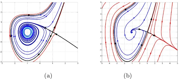
(a) (b)
Figure 4: The solution using (a) (µ1, µ2) = (−1,1), (a) (µ1, µ2) = (−1,2)
point moves to the same direction. This phenomenon shows that, there is no fixed point.
Case 2: Using µ1 <0 (with some fixed points)
In the second case, the value of the parameters are fixed by µ2 = √−µ1,
namelyµ1 =−1 andµ2= 1. Based on the theory described previously, there
exist two fixed points, (−1,0) and (1,0). Some initial points are choose in the area both near and far away from fixed points.
(−1,0). It means that this fixed point is a stable fixed point, as depict in Figure (4) (a). On the other hand, the fixed point (1,0) is a unstable fixed point. As the initial point is (1,0), the iteration produce a constant number. The initial point (1.1,0) leads a path moving away from the fixed point (1,0). Compared with Figure (1), the results is appropriate.
Case 3: Using µ1 <0 and µ2 >√−µ1
In the case ofµ2 >√−µ1, namelyµ1 =−1 andµ2= 2, the result have the
same characteristic. Compared with the case of µ1 =−1 and µ2 = 1, the
paths leads to the fixed point faster, as depicted in Figure (4) (b).
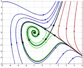
Case 4: Using µ1 <0 and µ2 <√−µ1
As the value ofµ2 = 0.5, the paths have different orientation compared with
the previous case, as shown in Figure (5). Currently, there exist two types of bifurcation and different orientation. There must be another bifurcation type between the orientation change.
Figure 5: The solution using (µ1, µ2) = (−1,0.5)
5. CONCLUSION
References
[1] A. Algaba, E. Freire, E. Gamero & A. J. Rodriguez-Luis. On the Takens-Bogdaniv Bifurcation in the Chua’s Equation. IEICE Trans. Fundamentals. Vol. E82-A, No.9, 1722-1728, (1999).
[2] F.A. Carrillo dan F. Verduce. Control of Planar Takens-Bugdanov Bi-furcation with Applications,Acta Appl. Math.vol. 105, 199-225, (2009).
[3] O. Y. Ababneh, R. Ahmad & E. S. Ismail: New Multi-step Runge-Kutta Method. Applied Mathematical Sciences, Vol. 3, no. 45, 2255-2262,(2009).
[4] E. Sermutlu. Comparison of runge-kutta methods of order 4 and 5 on lorenz equation,Journal of Arts and Sciences Say1 1/Mayis, (2004).
[5] N. Razali and R. R. Ahmad. Solving Lorenz System by Using Runge-Kutta Method. European Journal of Scientific Research, Vol.32 No.2, pp.241-251, (2009).
[6] J. Guckenheimer and P. Holmes. Nonlinear Oscillations, Dynamical Systems, and Bifurcations of Vector Fields. Applied Mathematical Sci-ences, vol. 42. Springer Verlag, (1993).
[7] S. Wiggins. Introduction to Applied Nonlinear Dynamical Systems and Chaos. New York: Springer-Verlag, (1990).
Tulus: Department of Mathematics, Faculty of Mathematics and Natural Sciences, University of Sumatera Utara, Medan 20155, Indonesia