Page 1 of 6
E-I
Q
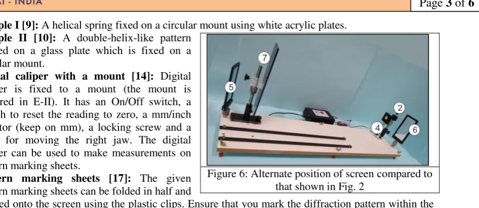
Figure 2: Apparatus for E-I
Figure 1: Photo 51
Diffraction due to Helical Structure
(Total marks: 10)
Introduction
The X-ray diffraction image of DNA (Fig. 1) taken in Rosalind Franklin’s
laboratory, famously known as “Photo 51”, became the basis of the discovery of
the double helical structure of DNA by Watson and Crick in 1952. This experiment will help you understand diffraction patterns due to helical structures using visible light.
Objective
To determine geometrical parameters of helical structures using diffraction.
List of apparatus
[1] Wooden platform [11] Plastic clips
[2] Laser source with its mount and base [12] Circular black stickers [3] DC regulated power supply for the Laser source [13] Mechanical pencil
[4] Sample holder with its base [14] Digital caliper with a mount [5] Left reflector (front coated mirror) [15] Plastic scale (30 cm) [6] Right reflector (front coated mirror) [16] Measuring tape (1.5 m) [7] Screen (10 cm x 30 cm) with its mount and base [17] Pattern marking sheets [8] Plane mirror (10 cm x 10 cm) [18] Laser safety goggles [9] Sample I (helical spring) [19] Battery operated flashlight
[10] Sample II
(double-helix-like pattern printed on glass plate)
Page 2 of 6
E-I
Q
Description of apparatus
Woodenplatform [1]: Apair of guiding rails, laser, reflectors, screen and sample mounts are rigidly fixed on it.
Laser source with its mount and base [2]: Laser source of wavelength ) is fixed in a metallic mount clamped to the base using a ball joint ([20] in Fig. 3) allowing
the adjustment in X-Y-Z directions. The laser body can be rotated and clamped using the top lock-in screw. The beam focus can be adjusted by rotating the front lens cap (red arrow in Fig. 3) to obtain a clear and sharp diffraction pattern.
DC regulated power supply [3]: The front panel has an intensity switch (high/low), socket for laser source connector and three USB sockets. The back panel has power switch and mains power socket (inset of Fig. 4).
Sample holder with its base [4]: Use the top locking screw to affix the samples in it (Fig. 3). The sample holder can be adjusted horizontally, vertically and rotated.
Left reflector [5]: Thisreflector is fixed to the platform (Fig. 5). Do not use the side marked X.
Right reflector [6]: This reflector is fixed to the platform and is removable (It will be removed in experiment E-II). Do not use the side marked X.
Screen with its mount [7]: The screen is mounted on ball joint and a base allowing rotational adjustments in all directions (Fig 5). The screen can be fixed as shown in Fig. 2 or Fig. 6 as required.
Figure 3: Laser source and sample holder. [20] Ball joint.
Figure 5: Left reflector and screen
Page 3 of 6
E-I
Q
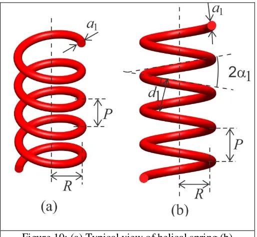
Sample I [9]: A helical spring fixed on a circular mount using white acrylic plates.
Sample II [10]: A double-helix-like pattern pattern marking sheets can be folded in half and
clipped onto the screen using the plastic clips. Ensure that you mark the diffraction pattern within the rectangular box.
Theory
A laser beam of wavelength , falling normally on a cylindrical wire of diameter , is diffracted in the direction perpendicular to the wire. The resulting intensity pattern as observed on a screen is shown in Fig. 7.
Figure 7: Schematic of the diffraction pattern due to single cylindrical
wire of diameter .Figure 8: Schematic of diffraction pattern due to two
cylindrical wires
The intensity distribution as a function of angle with the incident direction is given by
) ) * +
The central spot is bright and for other angles, when ) is zero, the intensity vanishes. Thus the intensity distribution has minimum at the angle , given by
Here refers to both sides of the central spot ( ).
The diffraction pattern due to two parallel identical wires kept at a distance d from each other (Fig. 8) is a combination of two patterns (diffraction due to a single wire and interference due to two wires). The resultant intensity distribution is given by,
) ) [ ]
where
Page 4 of 6
E-I
Q
For a screen placed at a large distance D from the wire, the positions of the minima on the screen are observed at
due to diffraction and at ( )
due to interference (where ). Similarly for a set of four identical wires (Fig. 9), the net intensity distribution is a combination of diffraction from each wire and interference due to pairs of wires and hence depends on , and . In other words, the combination of three different intensity patterns is observed.
Initial adjustments
1. Switch on the laser source and adjust both reflectors so that the laser spot falls on the screen. 2. Use the plastic scale and adjust the laser mount and reflectors such that the laser beam is parallel
to the wooden platform.
3. Make sure that the laser spot falls near the centre of the screen.
4. Switch off the laser source. Clamp the pattern marking sheet on the screen.
5. Clamp the given plane mirror on the screen using plastic clips and switch on the laser again. 6. Adjust the screen so that the laser beam retraces its path back to the laser source. Remove the
mirror once your alignment is completed.
7. Lights in the cubicle may be switched on/off as required.
Experiment
Part A: Determination of geometrical parameters of a helical spring
Sample I is a helical spring of radius and pitch made of a wire of uniform thickness as shown in Fig. 10(a). When viewed at normal incidence its projection is equivalent to two sets of parallel wires of the same thickness separated by distance and angle between them (Fig. 10(b)).
Figure 10: (a) Typical view of helical spring (b) Schematic diagram when viewed at normal incidence
Mount sample I in the sample holder ensuring that the spring is vertical.
Obtain a clear and sharp X-shaped diffraction pattern on the pattern marking sheet.
Page 5 of 6
E-I
Q
For this you may adjust
- laser beam focus (rotate lens cap)
- beam orientation (rotate the laser body so that only two turns of the spring are illuminated) - laser intensity (high/low switch on power supply)
- ambient light (by switching on or off cubicle light)
If the central maximum is very bright, you may stick circular black stickers on the pattern marking sheet to reduce scattering.
Tasks Description Marks
A1
Mark the appropriate positions (using given pencil [13]) of the intensity minima to determine and on the both sides of the central spot on the marking sheet. Please label your pattern-marking sheets as P-1, P-2 etc.
0.7
A2 Measure the appropriate distances using digital calipers and record them in Table A1 for
determining . 0.5
A3 Plot a suitable graph, label it Graph A1 and from the slope, determine . 0.7
A4 Measure the appropriate distances and record them in Table A2 for determining
.
0.8A5 Plot a suitable graph, label it Graph A2 and from the slope, determine . 0.6
A6 From the X-shaped pattern, determine the angle . 0.2
A7 Express in terms of and and calculate . 0.2
A8 Express in terms of and and calculate (neglect ). 0.2
Part B: Determination of geometrical parameters of double-helix-like pattern
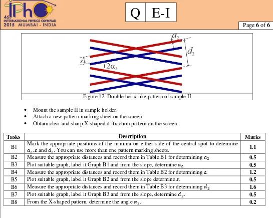
Figure 11(a) shows two turns of a double helix. Fig. 11(b) is a two-dimensional projection of this double helix when viewed at normal incidence. Each helix of thickness has an angle and perpendicular distance between turns. The separation between two helices is . Sample II is a double-helix-like pattern printed on glass plate (Fig. 12), whose diffraction pattern is similar to that of a double helix. In this part, you will determine the geometrical parameters of sample II.
Page 6 of 6
E-I
Q
Figure 12: Double-helix-like pattern of sample II
Mount the sample II in sample holder.
Attach a new pattern-marking sheet on the screen.
Obtain clear and sharp X-shaped diffraction pattern on the screen.
Tasks Description Marks
B1 Mark the appropriate positions of the minima on either side of the central spot to determine
and . You can use more than one pattern marking sheets. 1.1 B2 Measure the appropriate distances and record them in Table B1 for determining 0.5
B3 Plot suitable graph, label it Graph B1 and from the slope, determine . 0.5
B4 Measure the appropriate distances and record them in Table B2 for determining . 1.2 B5 Plot suitable graph, label it Graph B2 and from the slope determine . 0.5 B6 Measure the appropriate distances and record them in Table B3 for determining 1.6
B7 Plot suitable graph, label it Graph B3 and from the slope, determine . 0.5