Introduction to Management Science 9 th Edition by Bernard W. Taylor III. Chapter 9 Multicriteria Decision Making

(1)

Chapter 9 Multicriteria Decision Making

Introduction to Management Science

9

th

Edition

by Bernard W. Taylor III

(2)

Goal Programming

Interpretasi grafis dari Goal Programming

Solusi komputer masalh Goal Programming dengan QM for Windows and Excel

Analytical Hierarchy Process Scoring Models

(3)

Pembelajaran permasalahan dengan beberapa kriteria, multiple criteria,

bukan satu tujuan ketika membuat keputusan.

Tiga teknik yang dibahas: goal programming, analytical hierarchy process dan scoring models.

Goal programming adalah variasi dari program linier

mempertimbangkan lebih dari satu tujuan (goals) dalam fungsi tujuan. Analytical hierarchy process (AHP) merupakan memberian skor untuk setiap alternatif keputusan berdasarkan perbandingan masing-masing di bawah kriteria yang berbeda yang mencerminkan preferensi

pengambil keputusan..

Scoring models Model Scoring didasarkan pada teknik perkalian scoring yang relatif sederhana

(4)

Contoh Beaver Creek Pottery Company

Maksimalkan Z = $40x₁ + 50x₂ Batasan:

1x₁ + 2x₂  40 jam kerja

4x₁ + 3x₂  120 pon tanah liat x₁, x₂  0

Dimana: x₁ = Jumlah produksi mangkok x₂ = Jumlah produksi mug

(5)

Menambahkan tujuan (goals) dalam urutan kepentingan, perusahaan:

Tidak ingin menggunakan kurang dari 40 jam kerja per hari.

Ingin mencapai tingkat laba yang memuaskan dari $ 1.600 per hari.

Memilih untuk tidak menyimpan lebih dari 120 pon tanah liat di tangan setiap hari.

Ingin meminimalkan jumlah lembur.

(6)

Semua kendala tujuan adalah kesetaraan yang meliputi variabel deviasi d- dan d +.

Sebuah variabel deviasi positif (d +) adalah jumlah dimana tingkat tujuan terlampaui.

Variabel deviasi negatif (d-) adalah jumlah dimana tingkat tujuannya adalah di bawah tercapai.

Setidaknya satu atau kedua variabel deviasi dalam kendala tujuan harus sama dengan nol.

Fungsi tujuan dalam model goal programming untuk

meminimalkan penyimpangan dari tujuan masing-masing dalam urutan prioritas tujuan.

Goal Programming

Kendala Tujuan

(7)

Tujuan Jam Kerja:

x

₁

+ 2x

₂

+ d

₁-

_{- d}

1+

= 40 (jam/hari)

Tujuan Keuntungan:

40x

₁

+ 50 x

₂

+ d

₂ -

- d

₂ +

= 1,600 ($/hari)

Tujuan Material:

4x

₁

+ 3x

₂

+ d

₃ -

- d

₃ +

= 120 (tanah liat/hari)

Model Formulasi Goal Programming

Kendala Tujuan (1 of 3)

(8)

Kendala Tujuan Jam Kerja (prioritas 1 - kurang dari 40 jam kerja, prioritas 4 – minimum lembur ):

Minimalkan P₁d₁-_{, P}

4d1+

Kendala Penambahan Tujuan keuntungan (prioritas 2 -mencapai keuntungan sebesar $ 1.600):

Minimalkan P₁d₁-_{, P}

2d2-, P4d1+

Kendala Penambahan Tujuan Material (prioritas 3

-menghindari menjaga lebih dari 120 pon tanah liat di tangan): Minimalkan P₁d₁-, P₂d₂-, P₃d₃+, P₄d₁+

Model Formulasi Goal Programming

Fungsi Objektif (2 of 3)

(9)

Model Lengkap Goal Programming : Minimalkan P₁d₁-_{, P} 2d2-, P3d3+, P4d1+ batasan: x₁ + 2x₂ + d₁- _{- d} 1+ = 40 (jam kerja) 40x₁ + 50 x₂ + d₂- - d₂+ = 1,600 (keuntungan) 4x₁ + 3x₂ + d₃- _{- d} 3 + = 120 (tanah liat) x₁, x₂, d₁-_{, d} 1 +, d2 -, d2 +, d3 -, d3 +  0

Model Formulasi Goal Programming

Model Lengkap (3 of 3)

(10)

Mengubah keempat prioritas tujuan "batas lembur untuk 10 jam" bukannya meminimalkan lembur:

d₁- _{+ d}

4 - - d4+ = 10

minimalkan P₁d₁-_{, P}

2d2 -, P3d3 +, P4d4 +

Penambahan kelima prioritas tujuan "penting untuk mencapai tujuan untuk mug":

x₁ + d₅- _{= 30 mangkok}

x₂ + d₆- _{= 20 mug}

minimalkan P₁d₁-, P₂d₂-, P₃d₃+, P₄d₄+, 4P₅d₅- + 5P₅d₆

-Goal Programming

(11)

Goal Programming

Alternative Forms of Goal Constraints (2 of 2)

Model Lengkap dengan menambahkan Tujuan Baru:

Minimalkan P₁d₁-_{, P} 2d2-, P3d3+, P4d4+, 4P5d5- + 5P5d6 -batasan: x₁ + 2x₂ + d₁- _{- d} 1+ = 40 40x₁ + 50x₂ + d₂- _{- d} 2+ = 1,600 4x₁ + 3x₂ + d₃- _{- d} 3+ = 120 d₁+ _{+ d} 4- - d4+ = 10 x₁ + d₅- _{= 30} x₂ + d₆- _{= 20} x₁, x₂, d₁-_{, d} 1+, d2-, d2+, d3-, d3+, d4-, d4+, d5-, d6-  0

(12)

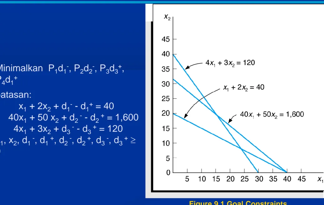
Minimalkan P₁d₁-_{, P} 2d2-, P3d3+, P₄d₁+ batasan: x₁ + 2x₂ + d₁- _{- d} 1+ = 40 40x₁ + 50 x₂ + d₂- _{- d} 2 + = 1,600 4x₁ + 3x₂ + d₃- _{- d} 3 + = 120 x₁, x₂, d₁-_{, d} 1 +, d2 -, d2 +, d3 -, d3 +  0

Figure 9.1 Goal Constraints

Goal Programming

(13)

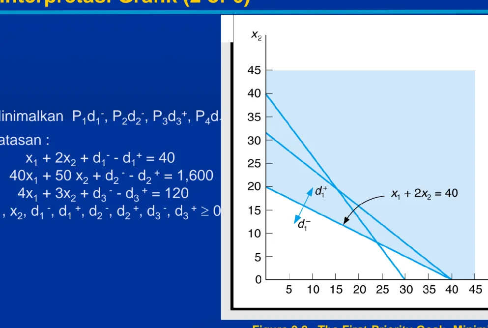
Figure 9.2 The First-Priority Goal: Minimize Minimalkan P₁d₁-_{, P} 2d2-, P3d3+, P4d1+ batasan : x₁ + 2x₂ + d₁- _{- d} 1+ = 40 40x₁ + 50 x₂ + d₂- _{- d} 2 + = 1,600 4x₁ + 3x₂ + d₃- _{- d} 3 + = 120 x₁, x₂, d₁-_{, d} 1 +, d2 -, d2 +, d3 -, d3 +  0

Goal Programming

Interpretasi Grafik (2 of 6)

(14)

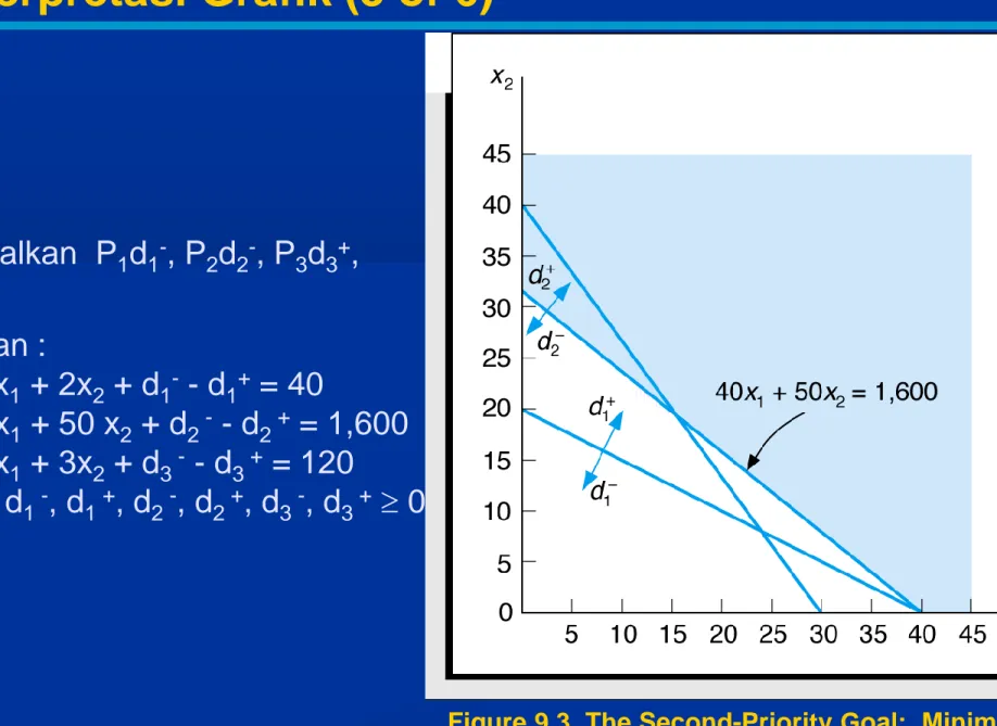
Figure 9.3 The Second-Priority Goal: Minimize Minimalkan P₁d₁-_{, P} 2d2-, P3d3+, P₄d₁+ batasan : x₁ + 2x₂ + d₁- _{- d} 1+ = 40 40x₁ + 50 x₂ + d₂- _{- d} 2 + = 1,600 4x₁ + 3x₂ + d₃- _{- d} 3 + = 120 x₁, x₂, d₁-_{, d} 1 +, d2 -, d2 +, d3 -, d3 +  0

Goal Programming

Interpretasi Grafik (3 of 6)

(15)

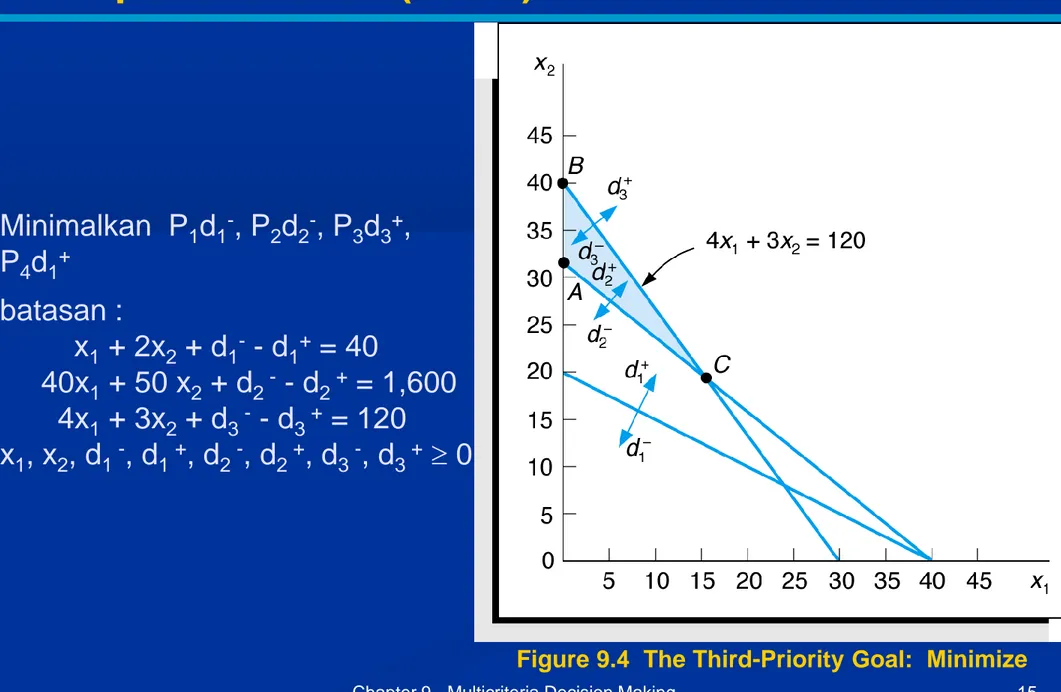
Figure 9.4 The Third-Priority Goal: Minimize Minimalkan P₁d₁-_{, P} 2d2-, P3d3+, P₄d₁+ batasan : x₁ + 2x₂ + d₁- _{- d} 1+ = 40 40x₁ + 50 x₂ + d₂- _{- d} 2 + = 1,600 4x₁ + 3x₂ + d₃- _{- d} 3 + = 120 x₁, x₂, d₁-_{, d} 1 +, d2 -, d2 +, d3 -, d3 +  0

Goal Programming

Interpretasi Grafik (4 of 6)

(16)

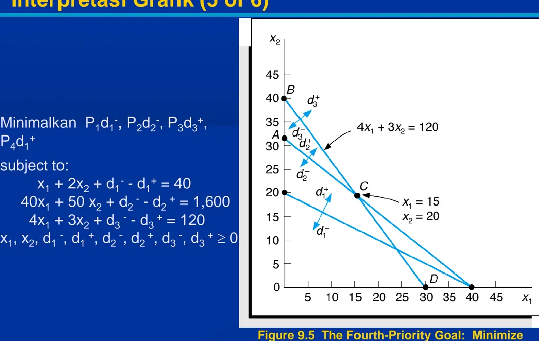
Figure 9.5 The Fourth-Priority Goal: Minimize Minimalkan P₁d₁-_{, P} 2d2-, P3d3+, P₄d₁+ subject to: x₁ + 2x₂ + d₁- _{- d} 1+ = 40 40x₁ + 50 x₂ + d₂- _{- d} 2 + = 1,600 4x₁ + 3x₂ + d₃- _{- d} 3 + = 120 x₁, x₂, d₁-_{, d} 1 +, d2 -, d2 +, d3 -, d3 +  0

Goal Programming

Interpretasi Grafik (5 of 6)

(17)

Solusi goal programming tidak selalu mencapai semua

tujuan dan tidak "optimal", mencapai yang terbaik atau yang paling memuaskan solusi yang mungkin.

Minimalkan P₁d₁-_{, P} 2d2-, P3d3+, P4d1+ batasan: x₁ + 2x₂ + d₁- _{- d} 1+ = 40 40x₁ + 50 x₂ + d₂- _{- d} 2 + = 1,600 4x₁ + 3x₂ + d₃- _{- d} 3 + = 120 x₁, x₂, d₁-_{, d} 1 +, d2 -, d2 +, d3 -, d3 +  0 Solusi: x₁ = 15 mangkok x₂ = 20 mug d₁- _{= 15 jam}

Goal Programming

Interpretasi Grafik (6 of 6)

(18)

Exhibit 9.4

Goal Programming

(19)

Exhibit 9.5

(20)

Exhibit 9.6

(21)

Minimize P₁d₁-, P₂d₂-, P₃d₃+, P₄d₄+, 4P₅d₅- + 5P₅d₆ -subject to: x₁ + 2x₂ + d₁- _{- d} 1+ = 40 40x₁ + 50x₂ + d₂- _{- d} 2+ = 1,600 4x₁ + 3x₂ + d₃- _{- d} 3+ = 120 d₁+ _{+ d} 4- - d4+ = 10 x₁ + d₅- _{= 30} x₂ + d₆- _{= 20} x₁, x₂, d₁-_{, d} 1+, d2-, d2+, d3-, d3+, d4-, d4+, d5-, d6-  0

Goal Programming

(22)

Exhibit 9.7

Goal Programming

(23)

Exhibit 9.8

Goal Programming

(24)

Exhibit 9.9

Goal Programming

(25)

Exhibit 9.10

Goal Programming

(26)

Exhibit 9.11

Goal Programming

(27)

AHP merupakan metode untuk merangking beberapa alternatif keputusan dan menyeleksi yang terbaik

pengambil keputusan mempunyai banyak tujuan dan kriteria yang mendasari keputusan.

Pengambil keputusan membuat keputusan berdasarkan bagaimana alternatif dibandingkan menurut beberapa kriteria.

Pembuat keputusan akan alternatif yang paling memenuhi kriteria keputusan nya.

AHP adalah proses untuk mengembangkan nilai numerik untuk menentukan peringkat masing-masing alternatif

keputusan berdasarkan seberapa baik alternatif memenuhi kriteria pembuat keputusan.

Analytical Hierarchy Process

Overview

(28)

Southcorp Development Company shopping mall site selection.

Three potential sites: Atlanta

Birmingham Charlotte.

Perbandingan kriteria untuk tempat : Customer market base.

Income level Infrastructure Transportation

Analytical Hierarchy Process

Contoh

(29)

Top of the hierarchy: the objective (select the best site).

Second level: how the four criteria contribute to the objective.

Third level: how each of the three alternatives contributes to each of the four criteria.

Analytical Hierarchy Process

Hierarchy Structure

(30)

Mathematically determine preferences for sites with respect to each criterion.

Mathematically determine preferences for criteria (rank order of importance).

Combine these two sets of preferences to mathematically derive a composite score for each site.

Select the site with the highest score.

Analytical Hierarchy Process

General Mathematical Process

(31)

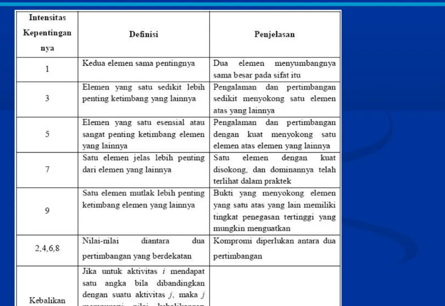
In a pairwise comparison, two alternatives are compared according to a criterion and one is preferred.

A preference scale assigns numerical values to different levels of performance.

Analytical Hierarchy Process

Pairwise Comparisons (1 of 2)

(32)

Table 9.1 Preference Scale for Pairwise Comparisons

Analytical Hierarchy Process

Pairwise Comparisons (2 of 2)

(33)

Income Level Infrastructure Transportation A B C                1 9 3 1/9 1 1/6 1/3 6 1                 1 1/7 1 7 1 3 1 1/3 1                 1 1/4 2 4 1 3 1/2 1/3 1 Customer Market Site A B C A B C 1 1/3 1/2 3 1 5 2 1/5 1

Analytical Hierarchy Process

Pairwise Comparison Matrix

A pairwise comparison matrix summarizes the pairwise comparisons for a criteria.

(34)

Customer Market Site A B C A B C 1 1/3 1/2 11/6 3 1 5 9 2 1/5 1 16/5

Customer Market

Site

A

B

C

A

B

C

6/11

2/11

3/11

3/9

1/9

5/9

5/8

1/16

5/16

Analytical Hierarchy Process

Developing Preferences Within Criteria (1 of 3)

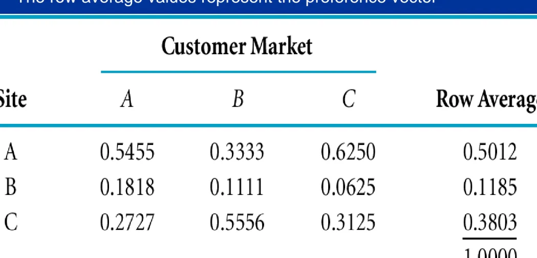
In synthesization, decision alternatives are prioritized with each criterion and then normalized:

(35)

Table 9.2 The Normalized Matrix with Row Averages

Analytical Hierarchy Process

Developing Preferences Within Criteria (2 of 3)

(36)

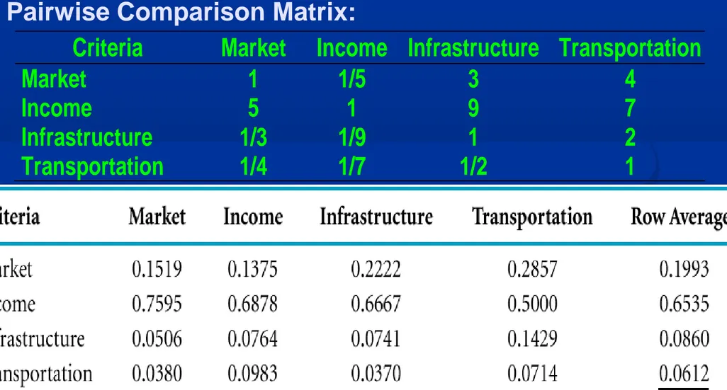
Table 9.3 Criteria Preference Matrix

Analytical Hierarchy Process

Developing Preferences Within Criteria (3 of 3)

Preference vectors for other criteria are computed similarly, resulting in the preference matrix

(37)

Criteria Market Income Infrastructure Transportation Market Income Infrastructure Transportation 1 5 1/3 1/4 1/5 1 1/9 1/7 3 9 1 1/2 4 7 2 1

Table 9.4 Normalized Matrix for Criteria with Row Averages

Analytical Hierarchy Process

Ranking the Criteria (1 of 2)

(38)

                        0.0612 0.0860 0.6535 0.1993

Analytical Hierarchy Process

Ranking the Criteria (2 of 2)

Preference Vector for Criteria:

Market Income

Infrastructure Transportation

(39)

Overall Score: Site A score = .1993(.5012) + .6535(.2819) + .0860(.1790) + .0612(.1561) = .3091 Site B score = .1993(.1185) + .6535(.0598) + .0860(.6850) + .0612(.6196) = .1595 Site C score = .1993(.3803) + .6535(.6583) + .0860(.1360) + .0612(.2243) = .5314 Overall Ranking:

Site

Score

Charlotte

Atlanta

Birmingham

0.5314

0.3091

0.1595

1.0000

Analytical Hierarchy Process

Developing an Overall Ranking

(40)

Analytical Hierarchy Process

Summary of Mathematical Steps

Develop a pairwise comparison matrix for each decision alternative for each criteria.

Synthesization

Sum the values of each column of the pairwise comparison matrices.

Divide each value in each column by the corresponding column sum.

Average the values in each row of the normalized matrices. Combine the vectors of preferences for each criterion.

Develop a pairwise comparison matrix for the criteria. Compute the normalized matrix.

Develop the preference vector.

Compute an overall score for each decision alternative Rank the decision alternatives.

(41)

Analytical Hierarchy Process: Consistency (1 of 3)

Consistency Index (CI): Check for consistency and validity of multiple pairwise comparisons

Example: Southcorp’s consistency in the pairwise comparisons of the 4 site selection criteria

Step 1: Multiply the pairwise comparison matrix of the 4 criteria

by its preference vector

Market Income Infrastruc. Transp. Criteria Market 1 1/5 3 4 0.1993 Income 5 1 9 7 X 0.6535 Infrastructure 1/3 1/9 1 2 0.0860 Transportation 1/4 1/7 1/2 1 0.0612 (1)(.1993)+(1/5)(.6535)+(3)(.0860)+(4)(.0612) = 0.8328 (5)(.1993)+(1)(.6535)+(9)(.0860)+(7)(.0612) = 2.8524 (1/3)(.1993)+(1/9)(.6535)+(1)(.0860)+(2)(.0612) = 0.3474 (1/4)(.1993)+(1/7)(.6535)+(1/2)(.0860)+(1)(.0612) = 0.2473

(42)

Analytical Hierarchy Process: Consistency (2 of 3)

Step 2: Divide each value by the corresponding weight from the

preference vector and compute the average 0.8328/0.1993 = 4.1786 2.8524/0.6535 = 4.3648 0.3474/0.0860 = 4.0401 0.2473/0.0612 = 4.0422 16.257 Average = 16.257/4 = 4.1564

Step 3: Calculate the Consistency Index (CI)

CI = (Average – n)/(n-1), where n is no. of items compared CI = (4.1564-4)/(4-1) = 0.0521

(43)

Analytical Hierarchy Process: Consistency (3 of 3)

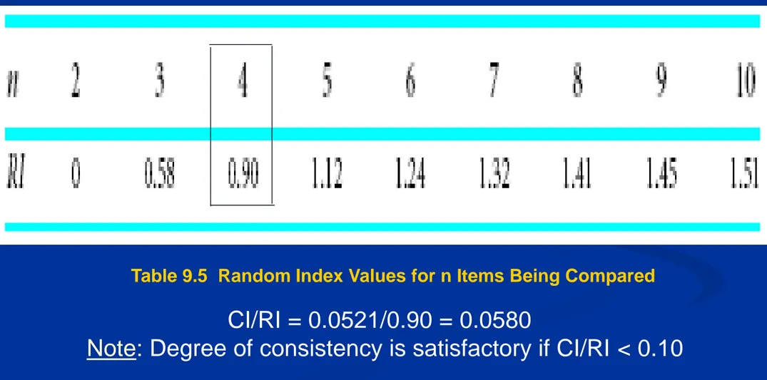
Step 4: Compute the Ratio CI/RI

where RI is a random index value obtained from Table 9.5

Table 9.5 Random Index Values for n Items Being Compared

CI/RI = 0.0521/0.90 = 0.0580

(44)

Exhibit 9.12

Analytical Hierarchy Process Excel Spreadsheets (1 of 4)

(45)

Exhibit 9.13

(46)

Exhibit 9.14

(47)

Exhibit 9.15

(48)

Each decision alternative graded in terms of how well it satisfies the criterion according to following formula:

S_i = g_ijw_j where:

w_j = a weight between 0 and 1.00 assigned to criterion j; 1.00 important, 0 unimportant; sum of total weights

equals one.

g_ij = a grade between 0 and 100 indicating how well alternative i satisfies criteria j; 100 indicates high

satisfaction, 0 low satisfaction.

Scoring Model

Overview

(49)

Mall selection with four alternatives and five criteria:

S₁ = (.30)(40) + (.25)(75) + (.25)(60) + (.10)(90) + (.10)(80) = 62.75 S₂ = (.30)(60) + (.25)(80) + (.25)(90) + (.10)(100) + (.10)(30) = 73.50 S₃ = (.30)(90) + (.25)(65) + (.25)(79) + (.10)(80) + (.10)(50) = 76.00 S₄ = (.30)(60) + (.25)(90) + (.25)(85) + (.10)(90) + (.10)(70) = 77.75

Mall 4 preferred because of highest score, followed by malls 3, 2, 1.

Grades for Alternative (0 to 100) Decision Criteria

Weight

(0 to 1.00) Mall 1 Mall 2 Mall 3 Mall 4 School proximity

Median income Vehicular traffic Mall quality, size Other shopping 0.30 0.25 0.25 0.10 0.10 40 75 60 90 80 60 80 90 100 30 90 65 79 80 50 60 90 85 90 70

Scoring Model

Example Problem

(50)

Exhibit 9.16

Scoring Model

Excel Solution

(51)

Goal Programming Example Problem

Problem Statement

Public relations firm survey interviewer staffing requirements determination.

One person can conduct 80 telephone interviews or 40 personal interviews per day.

$50/ day for telephone interviewer; $70 for personal interviewer. Goals (in priority order):

At least 3,000 total interviews.

Interviewer conducts only one type of interview each day. Maintain daily budget of $2,500.

At least 1,000 interviews should be by telephone.

Formulate a goal programming model to determine number of

interviewers to hire in order to satisfy the goals, and then solve the problem.

(52)

Purchasing decision, three model alternatives, three decision criteria.

Pairwise comparison matrices:

Prioritized decision criteria:

Price Bike X Y Z X Y Z 1 1/3 1/6 3 1 1/2 6 2 1 Gear Action Bike X Y Z X Y Z 1 3 7 1/3 1 4 1/7 1/4 1 Weight/Durability Bike X Y Z X Y Z 1 1/3 1 3 1 2 1 1/2 1

Criteria Price Gears Weight Price Gears Weight 1 1/3 1/5 3 1 1/2 5 2 1

Analytical Hierarchy Process Example Problem

Problem Statement

(53)

Step 1: Develop normalized matrices and preference

vectors for all the pairwise comparison matrices for criteria.

Price

Bike X Y Z Row Averages

X Y Z 0.6667 0.2222 0.1111 0.6667 0.2222 0.1111 0.6667 0.2222 0.1111 0.6667 0.2222 0.1111 1.0000 Gear Action

X Y Z 0.0909 0.2727 0.6364 0.0625 0.1875 0.7500 0.1026 0.1795 0.7179 0.0853 0.2132 0.7014 1.0000

Analytical Hierarchy Process Example Problem Problem Solution (1 of 4)

(54)

Weight/Durability

X Y Z 0.4286 0.1429 0.4286 0.5000 0.1667 0.3333 0.4000 0.2000 0.4000 0.4429 0.1698 0.3873 1.0000 Criteria

Bike Price Gears Weight

X Y Z 0.6667 0.2222 0.1111 0.0853 0.2132 0.7014 0.4429 0.1698 0.3873

Step 1 continued: Develop normalized matrices and

preference vectors for all the pairwise comparison matrices for criteria.

(55)

Step 2: Rank the criteria. Price Gears Weight                  0.1222 0.2299 0.6479

Criteria Price Gears Weight Row Averages Price Gears Weight 0.6522 0.2174 0.1304 0.6667 0.2222 0.1111 0.6250 0.2500 0.1250 0.6479 0.2299 0.1222 1.0000

(56)

Step 3: Develop an overall ranking. Bike X Bike Y Bike Z Bike X score = .6667(.6479) + .0853(.2299) + .4429(.1222) = .5057 Bike Y score = .2222(.6479) + .2132(.2299) + .1698(.1222) = .2138 Bike Z score = .1111(.6479) + .7014(.2299) + .3873(.1222) = .2806

Overall ranking of bikes: X first followed by Z and Y (sum of scores equal 1.0000).                                          1222 . 0 2299 . 0 6479 . 0 3837 . 0 7014 . 0 1111 . 0 1698 . 0 2132 . 0 2222 . 0 4429 . 0 0853 . 0 6667 . 0

(57)